Article

On the Choice of Metric to Calibrate Time-Invariant Ensemble Kalman Filter Hyper-Parameters for Discharge Data Assimilation and Its Impact on Discharge Forecast Modelling

Département de Genie Civil et de Genie du Bâtiment, Université de Sherbrooke, Sherbrooke, QC J1K 2R1, Canada
*
Author to whom correspondence should be addressed.
Hydrology 2021, 8(1), 36; https://doi.org/10.3390/hydrology8010036
Submission received: 30 December 2020 / Revised: 12 February 2021 / Accepted: 20 February 2021 / Published: 24 February 2021

Abstract

:
An important step when using some data assimilation methods, such as the ensemble Kalman filter and its variants, is to calibrate its parameters. Also called hyper-parameters, these include the model and observation errors, which have previously been shown to have a strong impact on the performance of the data assimilation method. Many metrics can be used to calibrate these hyper-parameters but may not all yield the same optimal set of values. The current study investigated the importance of the choice of metric used during the hyper-parameter calibration phase and its impact on discharge forecasts. The types of metrics used each focused on discharge accuracy, ensemble spread or observation-minus-background statistics. The calibration was performed for the ensemble square root Kalman filter over two catchments in Canada using two different hydrologic models per catchment. Results show that the optimal set of hyper-parameters depended heavily on the choice of metric used during the calibration phase, where data assimilation was applied. These sets of hyper-parameters in turn produced different hydrologic forecasts. This influence was reduced as the forecast lead time increased, because of not applying data assimilation in the forecast mode, and accordingly, convergence of model state ensembles produced in the calibration phase. However, the influence could remain considerable for a few days up to multiple weeks depending on the catchment and the model. As such, a preliminary analysis would be recommended for future studies to better understand the impact that metrics can have within and outside the bounds of hyper-parameter calibration.

1. Introduction

Accurate streamflow simulation has been always a high priority to water resources scientists and decision makers for a more reliable streamflow prediction. Numerous hydrological models, varying in structure and hydrological conceptualization, were developed to represent the hydrological processes over catchments that are affected by various hydrological and climatological characteristics. Yet, their performance in streamflow prediction comes with uncertainties rooted in forcing data, parameters, and model structure. To compensate for these uncertainties, post-processing and data assimilation methods have drawn the interest of hydrologists. While the former methods modify ensemble streamflow prediction (ESP) based on historical observed and simulated streamflow records, the latter methods update model states are based on available observations. Although various post-processing methods have been developed to improve ESP of single models (such as event bias correction method [1], quantile mapping method [2], and forecast ensemble calibration method [3]) and to combine ESPs of multiple models while respecting each model performance (such as quantile model averaging (QMA; [4]), and Bayesian model averaging (BMA; [5]), the necessity of data assimilation systems has been highlighted for the accuracy of the ensemble forecast regardless of post-processing implementation [6].
Data assimilation techniques are becoming more widespread in hydrologic modelling as more data become available. In particular, the value of the ensemble Kalman filter (EnKF; [7]) and its variants to improve discharge simulation has been shown repeatedly [8,9,10,11,12,13]. A conclusion often repeated in these studies is the importance of properly specifying the method’s own set of parameters, often called hyper-parameters, such as model and observation errors. Furthermore, [14] report that transparently quantifying observation and model errors are a bottleneck in using data assimilation for operational hydrologic forecasting. Different approaches have been developed to adjust these hyper-parameters in a transparent manner. The traditional way is an adjustment that aims to optimize a metric [15] resulting in hyper-parameters that are fixed in time, but there are also adaptive methods that allow hyper-parameters to evolve over time [16,17,18]. Though adaptive methods allow hyper-parameters to evolve over time, they do not necessarily reduce the number of hyper-parameters to calibrate.
Different metrics have been used across studies to calibrate these hyper-parameters, particularly for the EnKF and its variants. For example, [13,19] use metrics that focus on the accuracy of the hydrologic ensemble or its mean, while [8,12] use a metric that focuses on the representativeness of the hydrologic ensemble spread. Other studies, such as [11,20], use metrics tailored for data assimilation purposes by focusing on analysis increments or related properties. While some properties may be more important to one community, such as the data assimilation community, it is often not the most relevant property according to another community, such as many decision makers. For example, large reservoir managers may prioritize the evaluation of a hydrologic ensemble forecast’s performance based on the bias of the ensemble mean over a flooding period rather than based on the specified observation and model errors matching their true errors. This could be in contrast with the data assimilation community, which could favor the latter property since it is an underlying assumption for the proper use of many data assimilation methods, including the EnKF and its variants.
Ideally, all types of useful metrics should be improved. However, adjusting hyper-parameters specific to a data assimilation method in order to optimize a particular metric may potentially lead to a decrease in performance according to another. This is analogous to the procedure of calibrating parameters specific to a hydrologic model, which have been shown to have an impact on the parameters obtained and therefore on the behavior of the resulting model [21,22]. This can cause some ambiguity as to which metric to prioritize and raises questions about its importance on model performance for streamflow modelling and forecasting. Few studies assessing this impact in hydrology have been published, particularly in a context of discharge forecasting. Ref. [23] addressed the issue of using a spread-sensitive metric not supported by probability theory. The use of an incorrect equation led to a systematic underestimation of ensemble spread as a function of forecast lead time. Ref. [19] also presented some challenges faced when implementing the EnKF for lumped models over catchments in Quebec, Canada. The existence of a tradeoff between two metrics used to calibrate EnKF-specific hyper-parameters was shown when calibrating a single set of hyper-parameters over a large number of catchments. Nevertheless, the focus of studies regarding the effect of hyper-parameters calibration on the discharge forecasting’s performance was mainly on calibrating hyper-parameter sets based on a specific metric or two [8,24]. Owing to the earlier discussion, as different metrics prioritize different aspects of the discharge simulation, such as accuracy, uncertainty representativeness and bias quantification (the aspect of interest may vary from one community to another), a detailed study assessing the effect of different metrics on the discharge forecasting’s performance would be of great help to the water resources community.
Accordingly, the current study wished to investigate this feature in greater detail for individual catchments using different models and various metrics. Specifically, the objective of this study was to evaluate the impact that the choice of metric used to calibrate EnKF hyper-parameters can have on hydrologic discharge forecasting. An approach based on fixed hyper-parameters with respect to time was used to reduce complexity of the calibration and focus on the effect of hyper-parameters themselves.
The remainder of the article is divided into three parts. Section 2 presents the catchments, the hydrologic models, the EnKF and its application, the procedure used to generate forecasts, and the metrics. Section 3 presents the results, followed by a discussion for the calibration of the EnKF hyper-parameters and the hydrologic forecasts of various data assimilation scenarios. Section 4 provides some concluding remarks.

2. Materials and Methods

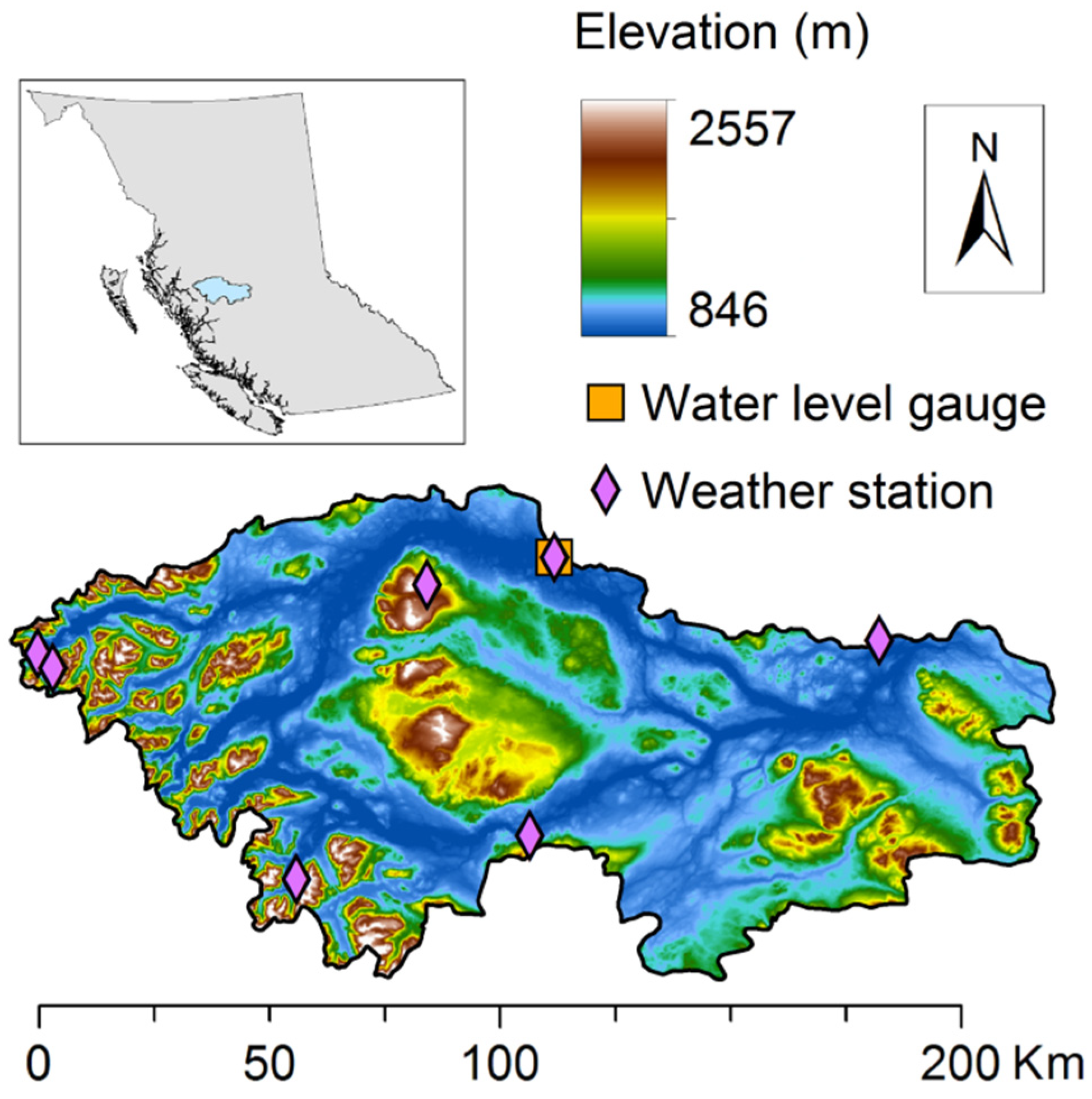
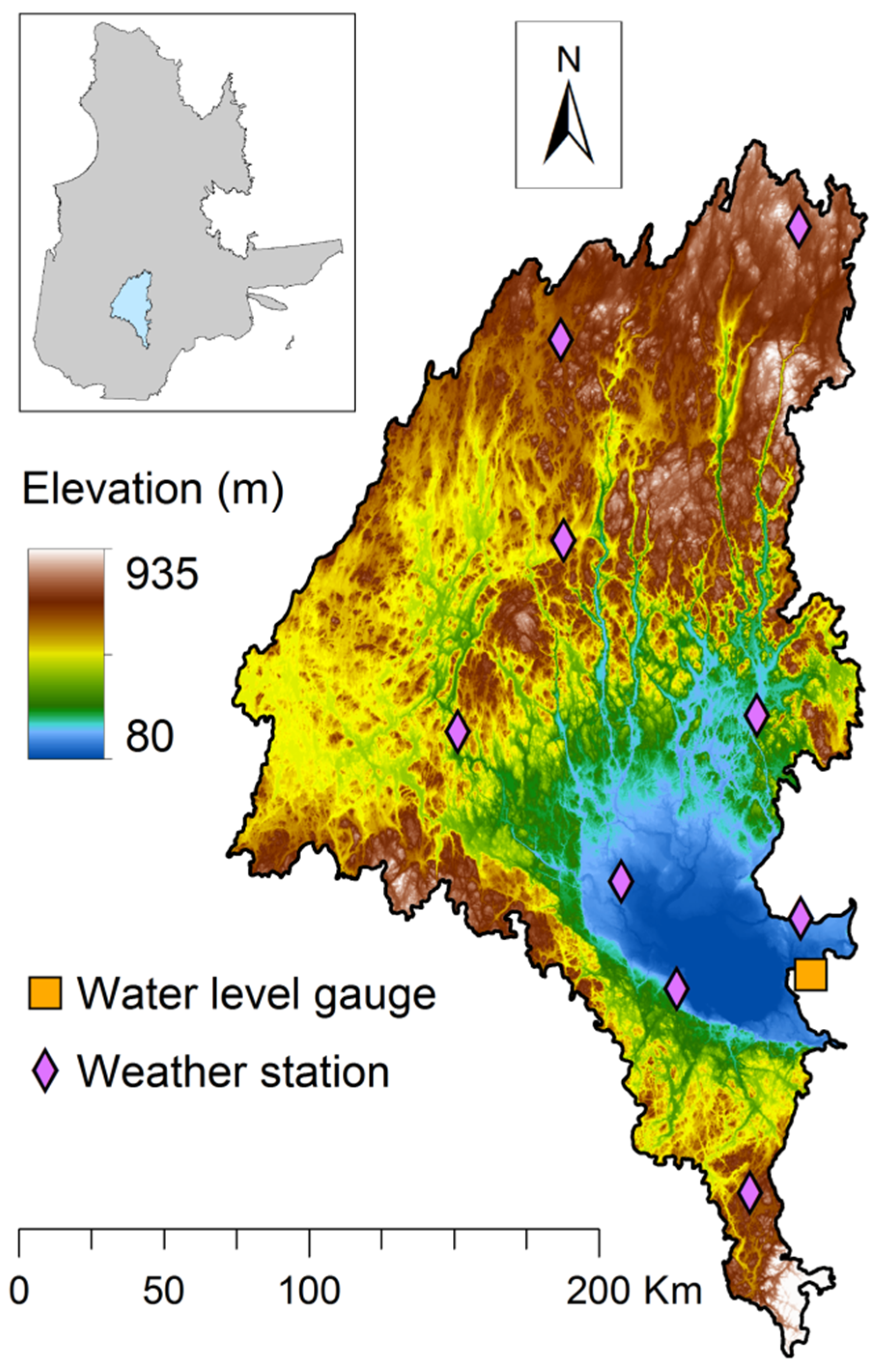
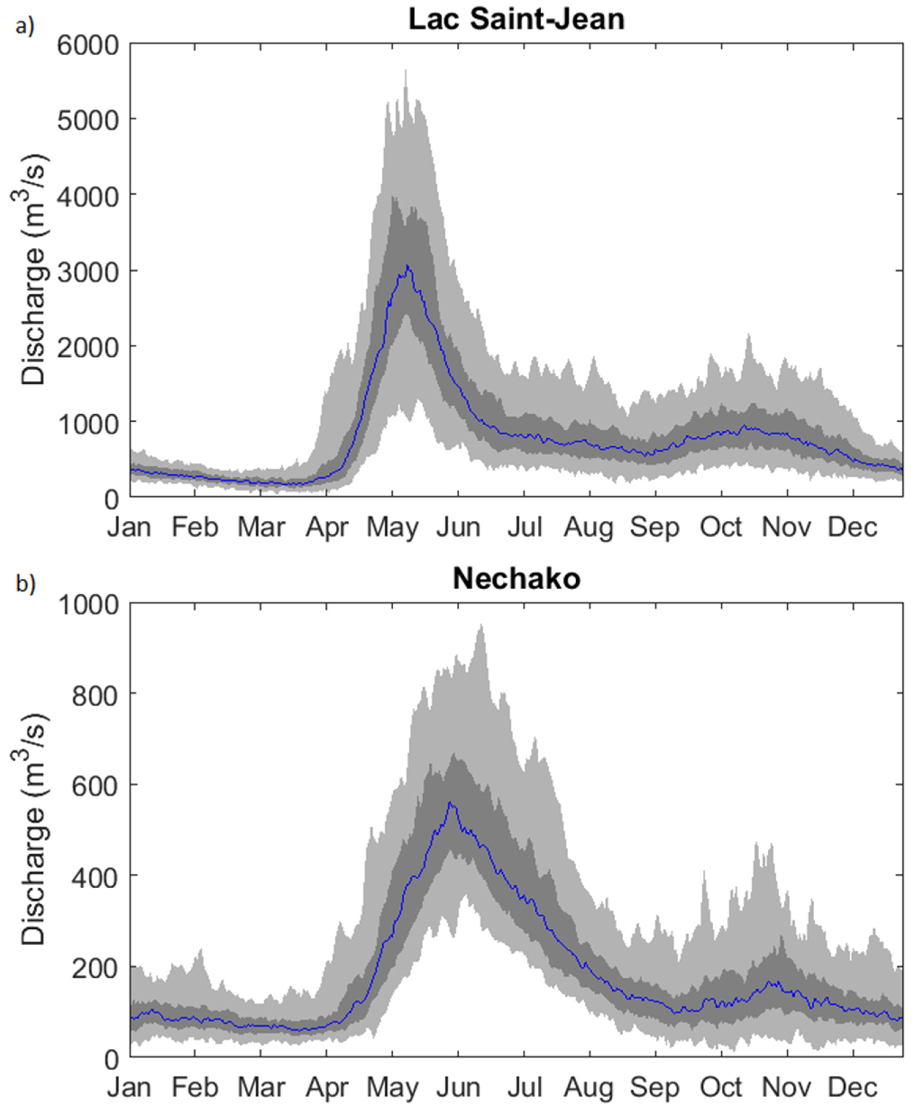
2.1. Study Catchments

Two catchments located in Canada were used in the current study. Both of these catchments contain reservoirs managed by Rio Tinto, mainly for hydroelectricity production purposes.
The first was the 14,106 km2 catchment drained by the Nechako reservoir located by the Coast Mountains in British Columbia, Canada (Figure 1). It is a mainly forested, snow-dominated catchment, where an estimated 53% of the precipitation falls as snow. The difference in elevation between the highest and lowest point in the watershed is recorded at 1711 m. The measured annual precipitation ranges between 703 mm and 1218 mm with an average of 903 mm.
The second was the 45,406 km2 Lac Saint-Jean catchment in Quebec, Canada (Figure 2). It is also a predominantly forested catchment. The measured annual precipitation ranges between 763 mm and 1244 mm and averages at 1019 mm. However, the difference in elevation is less prominent than the Nechako catchment, reaching a maximum of 855 m, and though snow precipitation contributes much to the hydrology of the catchment (estimation at 35%), most precipitation falls as rain.
Each catchment contains a hydrometric station (orange square) that measures daily water levels. Knowing the volume of water routed to the penstocks and the spillway every day, net natural discharge (hereby simply referred as discharge) can be computed from the differences in water level at a daily time step. A three-day smoothing filter was applied to the resulting discharge data to avoid irregularities, such as negative values. The time periods covered by these data ranged from 1957 to 2016 for the Nechako catchment, and 1953 to 2017 for the Lac Saint-Jean catchment. Historical discharge is shown in Figure 3 for the Lac Saint-Jean and Nechako catchments, with mean discharges of 868 m3/s and 203 m3/s, respectively. The snowmelt period is generally later for Nechako catchment, but snowmelt for both catchments normally occurs between 1 April and 31 August.
Several weather stations are also located within and around each catchment (Figure 1 for Lac Saint-Jean, Figure 2 for Nechako; purple diamonds). These stations measure daily precipitation and air temperature only. These measurements are then interpolated through weighted average using of the inverse distance of the three nearest stations to produce a grid that is 10 km × 10 km for the Lac Saint-Jean catchment and 5 km × 5 km for the Nechako catchment. The stations are protected by an Alter-type shield to mitigate the effect of the wind on precipitation measurements. However, there are strong suspicions that the measurements considerably underestimate the real precipitation, particularly for solid precipitation. These suspicions arose from the difficulties in closing the water balance, as well the well-known issue of snowfall undercatch [25]. There is anecdotal evidence that reports events where rain and snow gauge measurements likely did not yield a representative measurement. One example of such events, described by a Rio Tinto employee (B. Larouche, personal communication), includes the case where sticky snow formed a large snowball around and over a gauge opening in the Nechako catchment during a storm, preventing further solid precipitation from entering the gauge and therefore not being accounted for by the gauge. Correcting such event-based biases is a difficult challenge to overcome without independent and reliable observations. Some corrections have been applied manually by Rio Tinto for some events to match the volume of water over the melt season, as measured at the reservoir by the hydrometric gauge. Though these corrections are not ideal, in the sense that they are somewhat subjective and applied inconsistently over time, they provide an improved modelling of discharge forecasts.

2.2. Hydrologic Models

Two different hydrologic models were used in this study. The first was the spatially distributed model CEQUEAU [26]. It is a conceptual model that uses reservoirs to simulate hydrological processes, such as a surface reservoir to simulate near-surface processes such as infiltration and evapotranspiration, a deeper reservoir to simulate groundwater and base flows, and a reservoir for lakes and swamps. Evapotranspiration was modelled using the [27] formulation, while snow-related processes were modelled using the snow model presented by [28]. Overall, CEQUEAU required only daily precipitation and temperature as input, as well as a set of parameters that needed to be calibrated. These parameters had previously been calibrated by Rio Tinto to match discharge for each catchment separately. Table 1 shows the parameters used with CEQUEAU.
The second model was the spatially lumped GR4J [30]. Like CEQUEAU, GR4J is also a reservoir-type conceptual model that requires only daily precipitation and temperature as input, with one conceptual reservoir to simulate vertical water movement and a second reservoir for routing water at the watershed outlet. However, the default model does not model evapotranspiration or snow-related processes. The evapotranspiration module implanted followed the [31] formulation, while the snow module was the same as the mixed degree-days-energy-balance model formulated in the HYDROTEL [32] hydrologic model. The parameters were calibrated using the dynamically dimensioned search (DDS; [33]) algorithm to match discharge for each catchment separately. The values for these parameters are shown in Table 2. As mentioned earlier, GR4J coupled with HYDROTEL’s snow module differs from the basic GR4J model as it also accounts for snow accumulation and melt processes. This may be the reason for some calibrated parameters falling beyond the 80% confidence interval of empirical parameter range acquired by applying basic GR4J on different catchments without snow-related processes [30]. Additionally, model parameters falling outside the 80% confidence interval as presented in [30] did not automatically imply their values must be rejected. The confidence interval provided by [30], was derived from the 0.1 and 0.9 percentiles of the distributions of model parameters obtained over a large sample of catchments, implying that parameters outside the range were obtained for a number of tested watersheds. Finally, since this coupled model has been rarely applied in other studies, representing its empirical parameter range might be erroneous, and thus, were disregarded.
Though both models share some similarities, they nonetheless each use a different formulation applied at different scales for most processes. Perhaps the most significant distinction between the two models is in the way they numerically discretize the watershed since CEQUEAU uses regular tiles, while GR4J is lumped.

2.3. Ensemble Kalman Filter and Ensemble Square Root Kalman Filter

The data assimilation method used in this study was the ensemble square root Kalman filter (EnSRF; [34]). Like its better-known alternative, the ensemble Kalman filter [7], the EnSRF is a sequential data assimilation scheme that produces an analysis using a weighted average between an observed state and a modelled state. The main distinction between the two approaches is that the EnKF requires an ensemble of observations, which introduces sampling errors, while the EnSRF uses the observation covariance matrix to account for the observation errors. Another advantage of EnSRF is that, as opposed to EnKF, it does not assume a linear relationship between observations and model states [15]. These advantages, however, are at the cost of additional computations that are mainly rooted in separately updating model states mean and variance according to their respective observational values using two Kalman gain factors instead of one. In addition, and analogous to EnKF, the required time for data assimilation to be implemented also rises as the model’s calculation units get finer (i.e., the hydrological model is distributed on a finer grid). However, in the case where few observations are assimilated simultaneously, this additional computation becomes negligible because of lighter covariance matrix calculation and simultaneous analysis process for all observations.
In order to apply the EnSRF, an ensemble of model runs of size   N is propagated in time ( t ) to represent model errors. From this ensemble of modelled states ( x t b ) and its mean ( x t b ¯ ), the model covariance matrix ( P t b ) at a time t can be computed as such:
P t b = 1 N 1 ( x t b x t b ¯ ) ( x t b x t b ¯ )
An observation covariance matrix ( R t ) is also required for every time step for which an observation ( y t ) is to be assimilated. However, unlike the traditional EnKF, R t is not computed in a similar manner to eq 1 since observations are not perturbed. Instead, the full covariance matrix at each time step must be provided in order to compute the traditional Kalman gain ( K t ):
K t = P t b H t ( H t P t b H t + R t ) 1
where H t is the observation operator that converts the model state into the observations space. Another feature of the EnSRF is the application of a separate gain ( K ˜ t ) applied to update deviations from the ensemble mean:
K ˜ t = P t b H t [ ( H t P t b H t + R t ) 1 ] ( H t P t b H t + R t + R t ) 1
The updated states ( x t a ) are finally computed following:
x t a = x t b + K t ( y t H t x t b ¯ ) K ˜ t ( H t x t b H t x t b ¯ )
In the case where only one observation is available, or if several observations are assimilated separately, the terms R t and H t P t b H t become scalars and Equation (4) can be simplified (a more detailed derivation is provided by [34]) to yield:
x t a = x t b + K t ( y t H t x t b ¯ ) ( 1 + R t H t P t b H t + R t ) K t ( H t x t b H t x t b ¯ )

2.4. Data Assimilation Experiment

The scenarios considered in this study are based on the assimilation of the discharge for the Nechako and Lac Saint-Jean catchment. This section provides details related to the procedure used to assimilate these observations.

2.4.1. Precipitation Ensemble Generation

The ensemble size used for all scenarios in the study consisted of 64 members. This size was found to be an acceptable trade-off between computing time and consistency between successive models runs [13].
The ensemble used to apply the EnSRF was generated by perturbing precipitation input. Since precipitation cannot be negative, and also in order to generate random values similar to normal distribution to respect EnSRF assumptions, a gamma distribution was used to respect the physical bound of precipitation values without introducing bias and while complying with EnSRF assumptions [12,13,35]. In addition, in order to perturb precipitation and observation, while making sure that the introduced noises followed a zero mean Gaussian distribution (EnSRF assumption), introduced noises to precipitation and observation needed to be proportional to their mean values [8]. Accordingly, at every time step, the mean ( μ p c p , t ) around which the distribution was centered was the observed precipitation value, while the variance ( σ p c p , t ) was considered to be a hyper-parameter that was a function of the mean:
σ p c p , t = ( α p c p μ p c p , t ) 2
where α p c p is a multiplicative hyper-parameter that must be greater or equal to 0. The hyper-parameter was considered constant in space, which is equivalent to using an infinite correlation length. The observation variance was defined in a similar way so that it was computed as a function of the observed value and a multiplicative parameter ( α Q ):
R t = ( α Q y t ) 2
Since every state variable for both CEQUEAU and GR4J depends on precipitation, using an ensemble of precipitation as input produced an ensemble of states, which could be updated via the EnSRF. Additional perturbations on the states or temperature input were not applied given that preliminary investigations showed this deteriorated the model performance and added unnecessary hyper-parameters to calibrate. Similarly, model-specific parameters were not perturbed to simplify the procedure and reduce the number of hyper-parameters to calibrate. Therefore, this study focused on calibration of two hyper-parameters, α p c p and α Q , that affected quantification of model and observation errors, respectively.

2.4.2. State Vector Configuration

In order to have an effect on future time steps, discharge data assimilation needed to update state variables. Since discharge was a model output and not a state variable, other variables needed to be added to the state vector. The details of the procedure applied to select the relevant variables can be found in [36]. The procedure relied mainly on choosing the best performing scenario among many different state vector configurations. For the CEQUEAU model, these variables included the level of the surface reservoir, which was the conceptual equivalent of soil moisture, and the level of the routing reservoir, which routed the available water to the outlet. For the GR4J model, the variables included in the state vector included the level of the surface and routing reservoirs, as well as the water contained in the nonlinear routing stores computed using unit hydrographs.
The various scenarios produced included the open loop, which was the case where no data were assimilated, and different values of α p c p and α Q for the assimilation of discharge observations.

2.5. Ensemble Forecasting

Once discharge was assimilated, hydrologic ensemble forecasts [37] were produced using a historical weather ensemble (climatology) as input in their respective model. For example, starting from the states generated from the assimilation of discharge on the 1st of January 2010, the hydrologic forecast for the next day used an ensemble of precipitation and temperature using observations from January 2nd of all the other years except 2010. All other available years, even those occurring after the forecast time, were used in order to keep the ensemble size constant. The initial states from which hydrologic forecasts were generated were the results of the EnSRF. Since no data assimilation occurred during the forecast process, the effect of the various data assimilation scenarios should have eventually diminished over a sufficiently long lead time and converged with the open loop. The difference in performance between the scenarios and the open loop should have reflected the impact of each data assimilation scenario.

2.6. Metrics

Several metrics were used to calibrate the hyper-parameters of α p c p and α Q , as well as to assess the performance of different data assimilation scenarios for hydrologic forecasts. Though the list of potential assessment tools was very large [38,39] and continued to grow, only a few are presented here, which were deemed sufficient for the purpose of this study.
The Nash–Sutcliffe efficiency or NSE [40] is a widespread metric used by hydrologists. It is a normalized ratio between the magnitude of the residual variance and the measured data variance. It is computed as shown:
NSE = 1 t = 1 T ( x t ¯ y t ) 2 t = 1 T ( y ¯ y t ) 2 ,
where x t ¯ is the ensemble-averaged simulated discharge, y ¯ is the time-averaged observed discharge and T is the total number of time steps. The range of the NSE is defined by (−∞, 1] and improves as the value increases.
The mean absolute flood bias (MAFB) measures the average tendency of the model to overestimate or underestimate the total volume of discharge cumulated over a specific period of time, in this case the flooding period due to snowmelt defined from April 1st to August 31st. It is computed as shown:
MAFB = 1 N y r 1 N y r | t = 1 N F ( x t ¯ y t ) t = 1 N F y t | 100 % ,
where N y r is the number of years considered in the simulation and N F is the number of time steps for each flooding period (153 days in this case). The MAFB is defined in the range (0, ∞), where 0 corresponds to a perfect fit between the observed and simulated volume of water over the flooding periods. The MAFB increases as differences arise between the simulated and observed volumes, whether it is positive (overestimation) or negative (underestimation).
The continuous ranked probability score or CRPS [41] is a metric adapted to ensembles. It measures the mean squared difference between the simulated ( F ( x t ) ) and observed ( F ( y t ) ) cumulative probability distribution of a variable as such:
CRPS = 1 T t = 1 T + ( F ( x t ) F ( y t ) ) 2 d x ,
The CRPS ranges from 0 to +∞, with a lower value corresponding to a more accurate forecast. For discharge, the CRPS has units of m3/s.
The normalized root mean square ratio (NRR; [42]) was also adapted to ensemble. It is defined as the normalized ratio between the time-averaged root mean square error (RMSE) of the ensemble mean and the mean RMSE of the ensemble members:
NRR = 2 q q + 1 1 T t = 1 T ( x ¯ t y t ) 2 1 q i = 1 q 1 T t = 1 T ( x t , i y t ) 2
where q is the ensemble size. The NRR ranges from 0 to +∞. It essentially measures the deviation from an ideal spread (NRR = 1), with values inferior to 1 indicating a spread that is too large and values greater than 1 indicating too little spread. Unlike the previous metrics, the NRR is not directly affected by the accuracy of the ensemble but focuses on the representativeness of its spread. This is an important aspect of forecasts, particularly for hydrological forecasting centers that use ensemble prediction systems in their decision-making process.
The last metric used was the consistency diagnostic on innovations presented by [43]. Under the assumptions of linearity of the observation operator ( H ) and no correlation between the observation errors and background errors, the following relation should be valid if the covariance of observation errors ( R ) and the covariance on background errors in observations space ( H B H T ) are correctly specified in the analysis:
E [ ( y t H x t ) ( y t H x t ) T ] = R + H B H T
The E [   ] operator takes the temporal mean of its input. Since only one type of observation is assimilated and no more than one observation is assimilated at any given time step, the covariance matrices reduce to scalar values. Rearranging this equation, we obtain a ratio ( D 1 ) that can range from 0 to +∞ and is equal to unity under ideal error specification:
D 1 = E [ ( y t H x ¯ t ) ( y t H x ¯ t ) T ] ( R + H B H T ) 1
This last metric is specific to data assimilation matters for which an improper assignment of errors can potentially lead to filter divergence [34]. It can be used to calibrate hyper-parameters but cannot be used in forecast mode since there are no observations to assimilate over the forecast at the time for which forecasts are emitted.

3. Results and Discussion

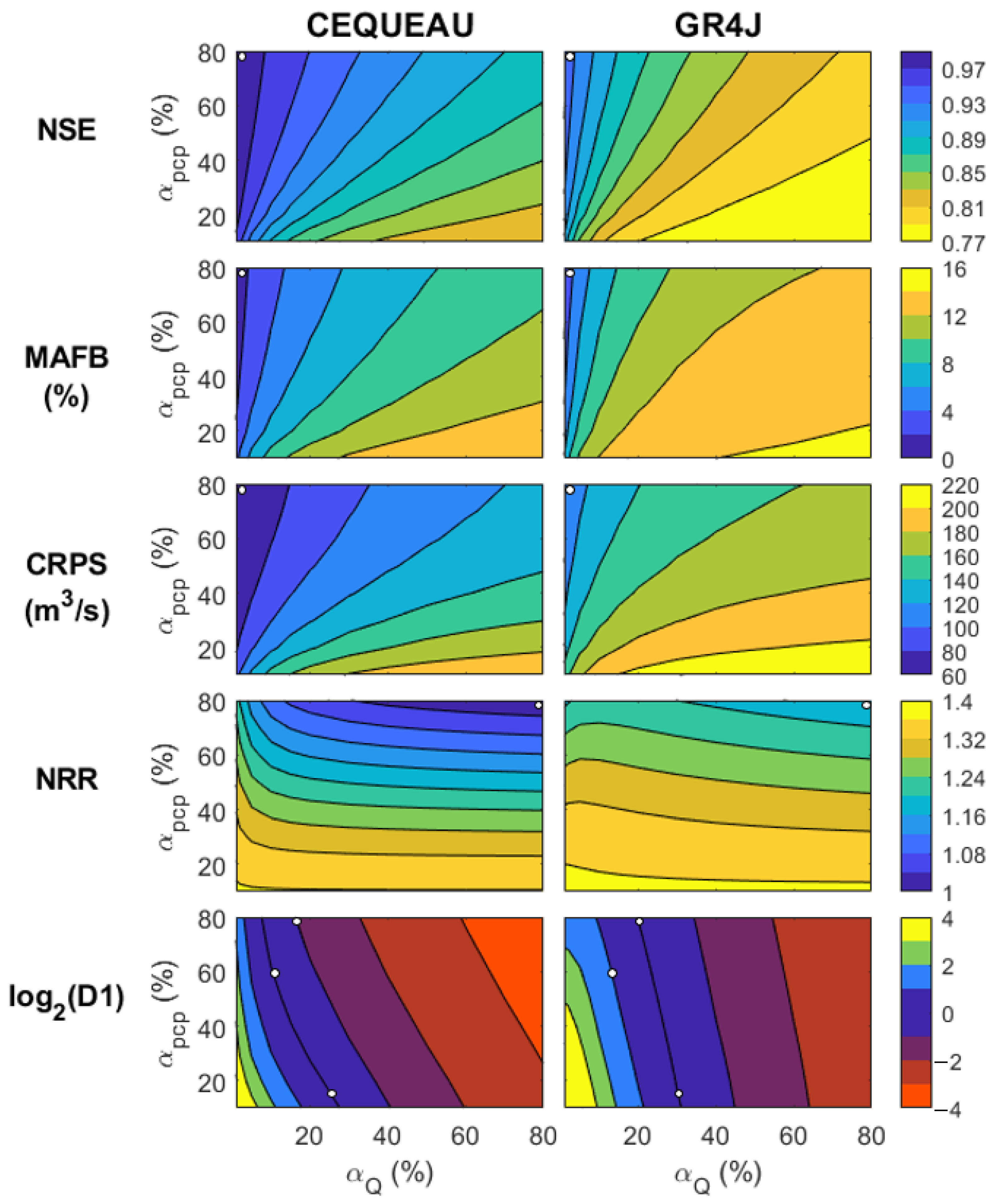
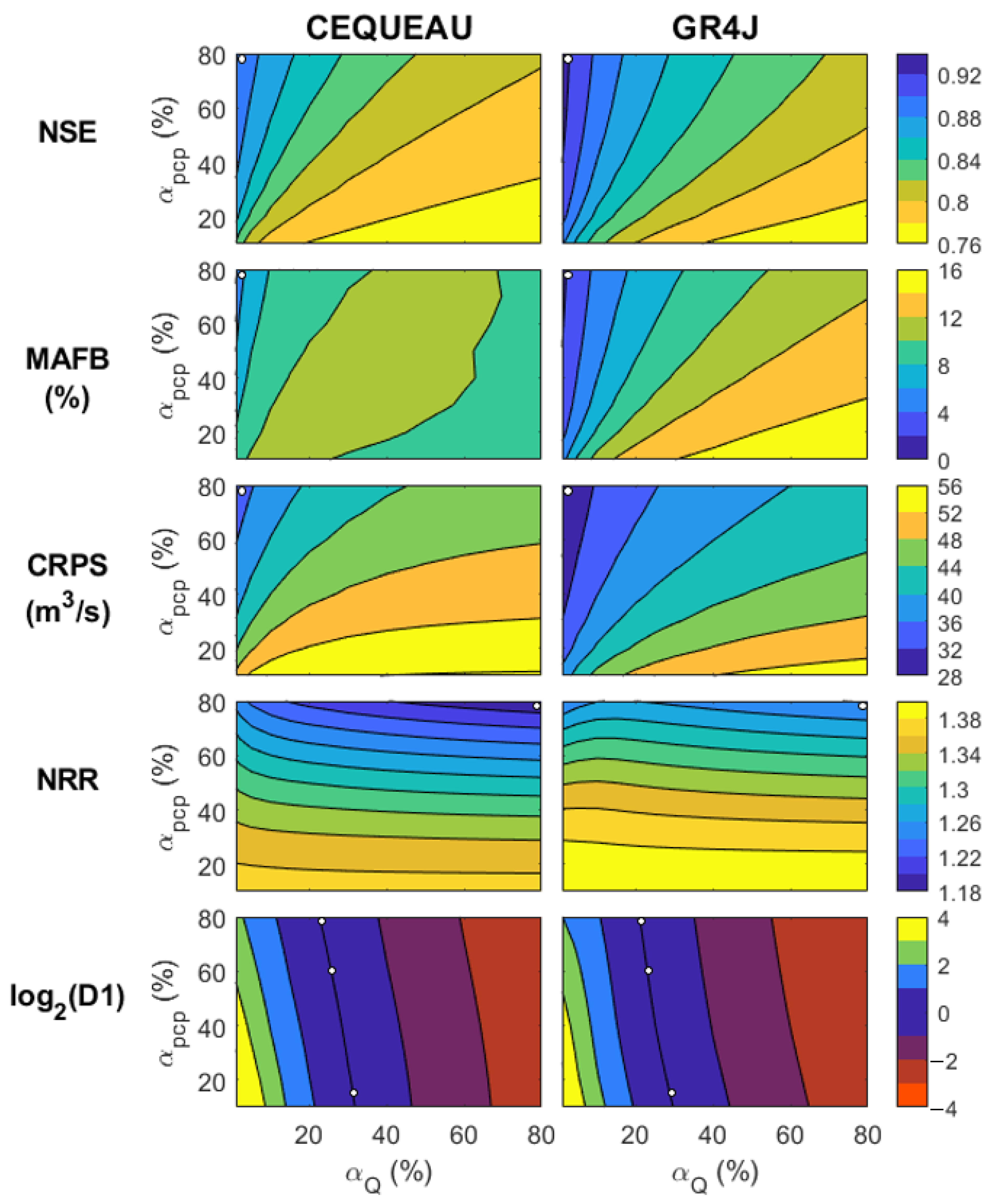
3.1. Calibration of EnSRF Hyper-Parameters

The data for the calibration of EnSRF hyper-parameters over the Lac Saint-Jean and Nechako catchments were respectively taken from the periods of 1 January 1955, to 31 December 1990, and 1 October 1992, to 30 September 2007, with the preceding two years being used as a warm-up period. First shown are the results of the calibration of the hyper-parameters α p c p and α Q over the Lac Saint-Jean (Figure 4) and Nechako (Figure 5) catchments. For both catchments, the performance of the models as a function of α p c p and α Q varied much according to all metrics shown. For example, the Nash–Sutcliffe efficiency could range from 0.76 to 0.94 and more, while the log2(D1) ranged from −4 to 4. The importance of proper specification of hyper-parameters shown here agrees with other studies that highlighted similar conclusions [15,44].
For the Lac Saint-Jean catchment (Figure 4), the overall portrait was similar across both hydrologic models, in the sense that the contour lines followed a similar pattern for each model and the optimal zones coincided. For the Nechako catchment (Figure 5), the portrait was once again similar across both models, though there were some differences. Notably, the MAFB contours for the GR4J model showed a positive gradient as α Q increased, while this only applied for the CEQUEAU model up to a certain region, after which the metric decreased in value (improved in performance).
The similarities across models seemed to indicate a low sensitivity of the calibration of the hyper-parameters to the choice of hydrologic model among the two shown here. This could be influenced by the type of observation assimilated and the relative similarities between the state vector used for each model. For example, assimilating a different type of observation, such as snow water equivalent, to update different state variables, such as simulated snow water equivalent, may have yielded different results. While some differences in absolute performance between the hydrologic models can be noted, as is also the case for the open loops, the question of which model performed best under various data assimilation schemes falls out of the scope of the current study.
As for the location of the optimal zones, they depended heavily on the choice of the metric used. The optimal zone, in ( α p c p , α Q ) coordinates, appeared to be (80,1), which were the upper and lower limits imposed during the calibration for the NSE, MAFB, and CRPS. This means that decreasing α Q or increasing α p c p could potentially further improve these metrics. In the opposite corners of these optimal zones were the zones of least performance. These results indicate that the model performed best when discharge observations were given large weights in the assimilation stage. The 1 % perturbation was likely an underestimation of the “true” observation error for discharge. This result could be the result of a suboptimal procedure in the generation of ensembles, such as avoiding perturbing model parameters and perturbing initial states beyond the spread produced by precipitation perturbations but was also influenced by the metrics’ focus on accuracy. Either way, these metrics were optimal around (80,1).
For the NRR, there was a local minimum (80,1) for the GR4J scenarios, but the optimal zones were nevertheless located at (80,80) for all scenarios, which was the upper limit used for both hyper-parameters. It is possible that the optimal zones lie beyond these limits, but pursuing this aspect would not be practical. High values of α p c p introduced heavy distortions on the resulting gamma distribution when compared with the ideal Gaussian distribution normally required for the EnSRF, as well as biases in the water balance due to the nonlinear relationship between precipitation and discharge. As for α Q , the limit where the hyper-parameter tended to +∞ resulted in the open loop. The current (80,80) result for the optimal zones and values of NRR consistently above 1 indicates that both models required additional spread. An important factor of this underestimation of ensemble spread may be the likely remaining bias in the precipitation input, even after manual corrections were applied. The assimilation of discharge observations reduced the resulting modelled discharge bias to some degree, but a method that acts directly on the precipitation input, such as one used in [9], could be more effective.
In the current setup, the variation found in the metrics up to this point was mainly monotonic, with the exception of the MAFB for the Nechako catchment and for the CEQUEAU model. For the D1, the optimal zone, that is for which the value equaled 0, followed a curve. The curve began near (10,30), went through a point near (60,25) and ended near (80,20) for all scenarios except the CEQUEAU model on the Lac Saint-Jean catchment, for which the two latter two points were closer to (60,10) and (80,8). This offers a set of solutions that is infinite in theory but can be reduced to a few points for practical purposes. This situation is analogous to the concept of equifinality well known to the hydrologic modelling community [45]. In this case, the situation could be avoided if the observed discharge error was fixed prior to running the scenarios, as is often done in studies (e.g., [9,10,13,44]). In this latter scenario, the calibration of the α P C P hyper-parameter would result in a single optimal solution. However, the full picture is shown here to demonstrate the complexity of the problem and the ambiguities that can arise when calibrating more than one hyper-parameter.
While a more complete pareto front could be determined using a multi-objective calibration approach [46], the results ultimately show that the optimal calibration solution depended on the choice of the metric used, which was the first step to reaching the study’s main objective. The calibration phase results indicate similar hyper-parameter pairs for metrics focused on the accuracy of the discharge simulation (NSE, MAFB, CRPS), regardless of the hydrological model used and the catchments considered. This suggests that satisfying one of these metrics should suffice for scientific projects mainly focusing on the accuracy of the discharge forecasts [12,13,47]. Similarly, hyper-parameter pairs were analogous for the metric focused on the uncertainty representativeness of the discharge simulation (NRR) for hydrological models and catchments considered. Satisfying this metric has been suggested for studies that prioritize the reliability of the discharge simulation while applying data assimilation [8,19]. However, attention should be paid in using these hyper-parameter pairs for other data assimilation sets, as the inner structure of the hydrological models, calibration algorithms, accuracy of the forcing and observation data, model states configuration can all affect the selected hyper-parameter pairs for different metrics. For instance, distributed physically based hydrological models with the capability of simulating more elaborate hydrological processes, while accounting for the heterogeneous processes over catchments, are expected to yield more accurate model states, and therefore, model states are given more weights through data assimilation implementation.
According to calibrated hyper-parameter pairs based on each metric, four sets of solutions were chosen to generate hydrologic forecast scenarios, along with reference scenarios, to quantify the impact of the calibration solutions on forecasts. As indicated in Figure 4 and Figure 5 using white dots, one of these scenarios was the (80,1) optimal point for the NSE-MAFB-CRPS combo, named the OptNBC scenario from now on. The second was the (80,80) optimal point according to the NRR metric, referred to as the OptNRR scenario. The other two scenarios fell on the optimal curve shown for the D1 metric. One was the (10,30) point named OptDQ since it had a larger value for α Q . This point was common to the curves of all cases shown in Figure 4 and Figure 5 for the D1 metric. The other scenario (OptPCP) had different values depending on the model and catchment since the upper end of the curves were not identical. The hyper-parameter values were (60,10) and (80,20) for CEQUEAU and GR4J over the Lac Saint-Jean catchment, and (60,25) and (80,20) for CEQUEAU and GR4J over the Nechako catchment, respectively. The scenarios are summarized in Table 3.

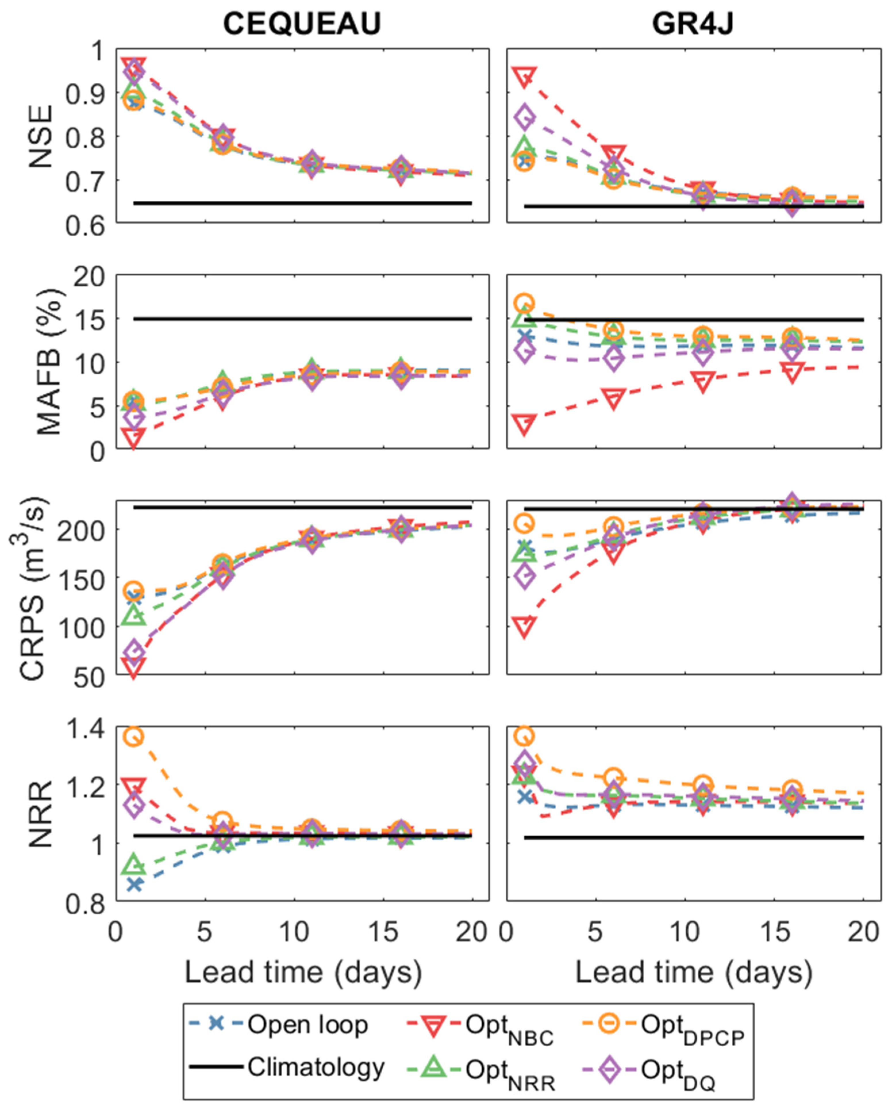
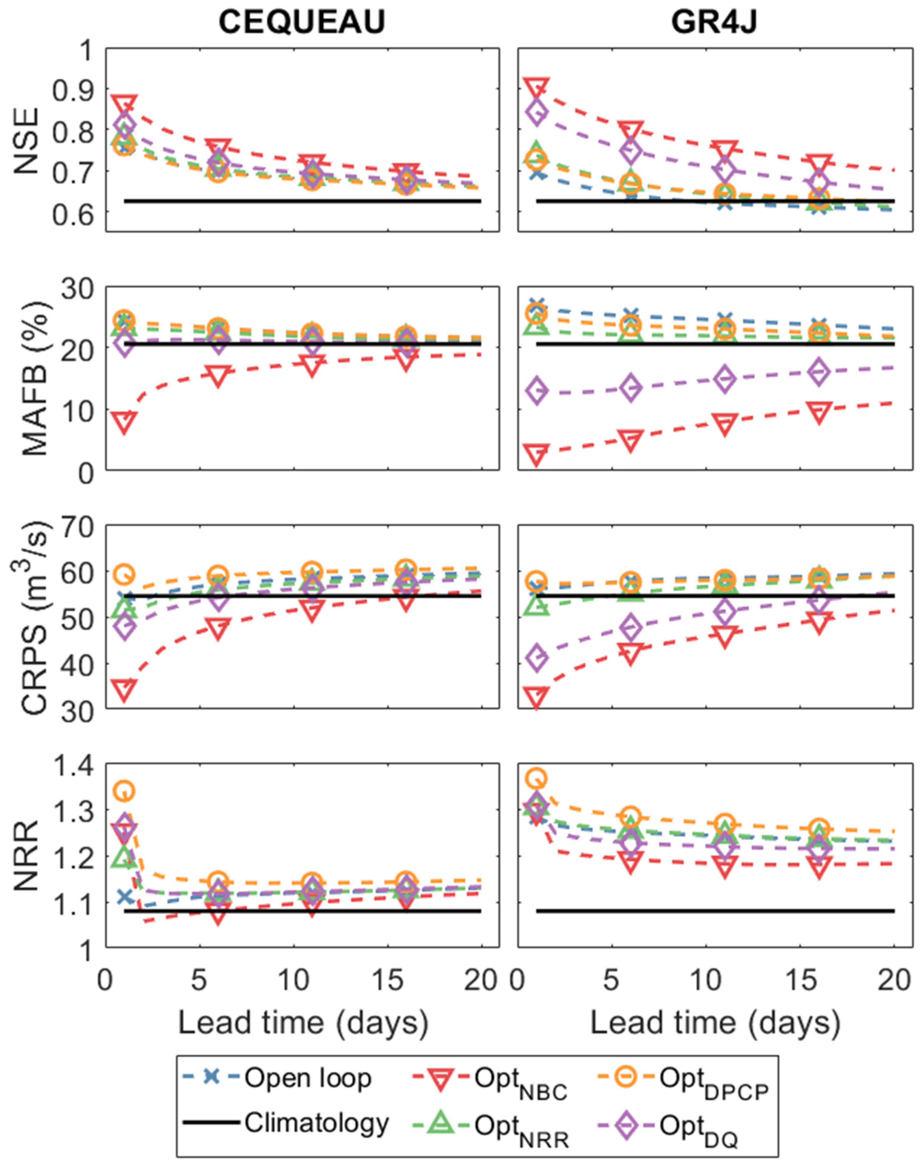
3.2. Discharge Forecasting

Forecasts were made for various scenarios over a different period than the calibration, spanning 1 January 1991, to 31 December 2017, for the Lac Saint-Jean catchment and 1 October 2007, to 30 September 2016, for the Nechako catchment. Note that these periods include every day of the year, including the winter and spring periods when snow accumulates and melt. Results for the Lac Saint-Jean and Nechako forecasts are shown in Figure 6 and Figure 7, respectively. The scenarios include the four sets of optimal hyper-parameters (OptNBC, OptNRR, OptDQ and OptPCP), as well as two different references; namely, the open loop and a historical discharge ensemble (climatology) which was comprised of all the observed discharge with the same day of the year as the forecasted day.
For the Lac Saint-Jean catchment (Figure 6), results show that the four data assimilation scenarios and the open loop performed generally better than the climatology for the NSE, the MAFB, and the CRPS, but not for the NRR. It was expected that the climatology should have been close to the ideal value (unity) and should have approached it when the sample size and the period for forecasts increased. For the climatology scenario, all metrics were independent of the forecast lead time because only the day of year of the forecast mattered. Since the climatological precipitation and temperature were used as the inputs to the forecast mode, it was expected that after a specific lead time, initial model states derived from data assimilation implementation under different scenarios for hyper-parameter calibration, would converge toward the climatological discharge. This lead time was the time length required for climatological weather inputs to negate initial model states derived from data assimilation. According to Figure 6, lead time of 1–20 days seem sufficient for four DA scenarios and the open loop to converge for NSE and CRPS metrics but not for the MAFB. Seeing that MAFB was computed only during the melt period, it was mainly affected by the amount of snow that accumulated over many months prior to melting. Using the climatological precipitation for a lead time of 1–20 days appears to be insufficient to converge back to the climatological snow water equivalent and therefore insufficient to converge back to the climatological discharge volume. The MAFB should have eventually converged to the climatology scenario with a sufficiently long lead time (many months). The improvement of the NRR as the lead time increases shows that the ensemble spread was becoming more representative of its error, but this was insufficient for GR4J, for which the ensemble spread remained too thin (NRR > 1).
For the Nechako catchment (Figure 7), the climatology was not surpassed as easily, even for the open loop. As shown by the poor performance of the open loop for the MAFB, this could have been influenced by the likely undercatch of snow precipitation, which fell more frequently in the Nechako catchment. The only scenario that improved forecasts for nearly all metrics and lead times, for both the climatology and the open loop, was the OptNBC, which minimized the ratio of observation error to model error.
The spread for each metric between the four data assimilation scenarios varied between models and catchments. Choosing to calibrate hyper-parameters using one metric or another can have an impact on forecasts that can last a few days to multiple weeks. Relative to the initial spread, the scenarios converged to similar values more slowly as a function of the forecast lead time for the Nechako catchment than the Lac Saint-Jean catchment, and more slowly for GR4J than the CEQUEAU. For the difference between models, it should be expected since the variables included in the state vector were different. For the difference between catchments, the additional snow in the Nechako catchment played an important role in the duration of the spread. Although the modelled snow–water equivalent was not included in the state vector and was therefore not updated through the Kalman gain, its spread was nonetheless affected by the hyper-parameter α p c p . Changes to snow–water equivalent mainly affect discharge during the spring, which occurs around the same time from year to year, as opposed to groundwater storage which affects discharge in the following days. Depending on the time of the year that the forecasts are generated, the changes to the snowpack can potentially affect discharge weeks or months later [13].

4. Conclusions

The study investigated the impact of the choice of metric on the EnSRF hyper-parameters calibration and its application for discharge forecasting. The calibration phase showed that the optimal set of hyper-parameters varied depending on the metric considered but was not strongly affected by the hydrologic models used and the catchment over which they were applied. It was shown that the choice of metric used during the calibration phase influenced discharge forecasts over a different period. This influence, regardless of the hydrological model and the catchment, diminished as the forecast lead time increased but remained substantial for lead times of a few days up to multiple weeks depending on the catchment and the model used. Careful attention and a preliminary analysis would be recommended for future studies when choosing a metric to optimize during the hyper-parameter calibration phase, as this choice can have a lasting impact on hydrologic forecasts. Some properties may be improved that could satisfy some underlying assumptions behind the data assimilation method, but this could also lead to a deterioration of other properties that may be of more practical interest to decision makers.
These results should not necessarily be generalized to all models, as the models used in this study were not representative of all hydrologic models, though they had many differences. The same caution should apply to the generalization over all catchments, especially since the catchments used in this study share many similarities, such as having snow cover for multiple months a year. The results are also possibly dependent on the setup used in the data assimilation approach. This includes the configuration of the state vector, the generation of ensembles, as well as the preprocessing and post-processing options. As such, expanding the works to include a wider variety of metrics, catchments, and models would be of interest for future studies, as well as investigating the effect of seasonality on the calibration of the EnKF hyper-parameters.

Author Contributions

Conceptualization, J.B., R.L. and M.T.; methodology, J.B., R.L. and M.T.; formal analysis, J.B.; writing—original draft preparation, J.B.; writing—review and editing, R.L., M.T. and S.F.; visualization, J.B. and S.F.; supervision, R.L.; funding acquisition, J.B., R.L. and M.T. All authors have read and agreed to the published version of the manuscript.

Funding

This work was supported by Rio Tinto and the Natural Sciences and Engineering Research Council of Canada (NSERC). Additional funding was obtained from the Fonds de recherche du Québec—Nature et technologies (FRQNT).

Data Availability Statement

Restrictions apply to the availability of these data. Data were obtained from Rio Tinto and are available from the authors with the permission of Rio Tinto.

Acknowledgments

We thank the staff at Rio Tinto for their collaboration in this study, providing useful insight, all of the data, and the hydrologic model CEQUEAU.

Conflicts of Interest

The authors declare no conflict of interest.

References

  1. Smith, J.A.; Day, G.N.; Kane, M.D. Nonparametric Framework for Long-range Streamflow Forecasting. J. Water Resour. Plan. Manag. 1992, 118, 82–92. [Google Scholar] [CrossRef]
  2. Hashino, T.; Bradley, A.A.; Schwartz, S.S. Evaluation of bias-correction methods for ensemble streamflow volume forecasts. Hydrol. Earth Syst. Sci. 2007, 11, 939–950. [Google Scholar] [CrossRef] [Green Version]
  3. Wood, A.W.; Schaake, J.C. Correcting Errors in Streamflow Forecast Ensemble Mean and Spread. J. Hydrometeorol. 2008, 9, 132–148. [Google Scholar] [CrossRef]
  4. Schepen, A.; Wang, Q.J. Model averaging methods to merge operational statistical and dynamic seasonal streamflow forecasts in Australia. Water Resour. Res. 2015, 51, 1797–1812. [Google Scholar] [CrossRef]
  5. Raftery, A.E.; Gneiting, T.; Balabdaoui, F.; Polakowski, M. Using Bayesian Model Averaging to Calibrate Forecast Ensembles. Mon. Weather Rev. 2005, 133, 1155–1174. [Google Scholar] [CrossRef] [Green Version]
  6. Bourgin, F.; Ramos, M.-H.; Thirel, G.; Andréassian, V. Investigating the interactions between data assimilation and post-processing in hydrological ensemble forecasting. J. Hydrol. 2014, 519, 2775–2784. [Google Scholar] [CrossRef]
  7. Evensen, G. Sequential data assimilation with a nonlinear quasi-geostrophic model using Monte Carlo methods to forecast error statistics. J. Geophys. Res. Space Phys. 1994, 99, 10143–10162. [Google Scholar] [CrossRef]
  8. Moradkhani, H.; Sorooshian, S.; Gupta, H.V.; Houser, P.R. Dual state–parameter estimation of hydrological models using ensemble Kalman filter. Adv. Water Resour. 2005, 28, 135–147. [Google Scholar] [CrossRef] [Green Version]
  9. Crow, W.T.; Ryu, D. A new data assimilation approach for improving runoff prediction using remotely-sensed soil moisture retrievals. Hydrol. Earth Syst. Sci. 2009, 13, 1–16. [Google Scholar] [CrossRef] [Green Version]
  10. Chen, F.; Crow, W.T.; Starks, P.J.; Moriasi, D.N. Improving hydrologic predictions of a catchment model via assimilation of surface soil moisture. Adv. Water Resour. 2011, 34, 526–536. [Google Scholar] [CrossRef]
  11. Trudel, M.; Leconte, R.; Paniconi, C. Analysis of the hydrological response of a distributed physically-based model using post-assimilation (EnKF) diagnostics of streamflow and in situ soil moisture observations. J. Hydrol. 2014, 514, 192–201. [Google Scholar] [CrossRef]
  12. Abaza, M.; Anctil, F.; Fortin, V.; Turcotte, R. Exploration of sequential streamflow assimilation in snow dominated watersheds. Adv. Water Resour. 2015, 80, 79–89. [Google Scholar] [CrossRef]
  13. Bergeron, J.M.; Trudel, M.; Leconte, R. Combined assimilation of streamflow and snow water equivalent for mid-term ensemble streamflow forecasts in snow-dominated regions. Hydrol. Earth Syst. Sci. 2016, 20, 4375–4389. [Google Scholar] [CrossRef] [Green Version]
  14. Liu, Y.; Weerts, A.H.; Clark, M.P.; Franssen, H.-J.H.; Kumar, S.V.; Moradkhani, H.; Seo, D.-J.; Schwanenberg, D.; Smith, P.; Van Dijk, A.I.J.M.; et al. Advancing data assimilation in operational hydrologic forecasting: Progresses, challenges, and emerging opportunities. Hydrol. Earth Syst. Sci. 2012, 16, 3863–3887. [Google Scholar] [CrossRef] [Green Version]
  15. Clark, M.P.; Rupp, D.E.; Woods, R.A.; Zheng, X.; Ibbitt, R.P.; Slater, A.G.; Schmidt, J.; Uddstrom, M.J. Hydrological data assimilation with the ensemble Kalman filter: Use of streamflow observations to update states in a distributed hydrological model. Adv. Water Resour. 2008, 31, 1309–1324. [Google Scholar] [CrossRef]
  16. Crow, W.T.; Reichle, R.H. Comparison of adaptive filtering techniques for land surface data assimilation. Water Resour. Res. 2008, 44, 1–12. [Google Scholar] [CrossRef] [Green Version]
  17. Leisenring, M.; Moradkhani, H. Analyzing the uncertainty of suspended sediment load prediction using sequential data assimilation. J. Hydrol. 2012, 468–469, 268–282. [Google Scholar] [CrossRef]
  18. Crow, W.T.; Yilmaz, M.T. The Auto-Tuned Land Data Assimilation System (ATLAS). Water Resour. Res. 2014, 50, 371–385. [Google Scholar] [CrossRef]
  19. Thiboult, A.; Anctil, F. On the difficulty to optimally implement the Ensemble Kalman filter: An experiment based on many hydrological models and catchments. J. Hydrol. 2015, 529, 1147–1160. [Google Scholar] [CrossRef] [Green Version]
  20. Waller, J.A.; Dance, S.L.; Lawless, A.S.; Nichols, N.K. Estimating correlated observation error statistics using an ensemble transform Kalman filter. Tellus A: Dyn. Meteorol. Oceanogr. 2014, 66, 23294. [Google Scholar] [CrossRef] [Green Version]
  21. Diskin, M.; Simon, E. A procedure for the selection of objective functions for hydrologic simulation models. J. Hydrol. 1977, 34, 129–149. [Google Scholar] [CrossRef]
  22. Jie, M.-X.; Chen, H.; Xu, C.-Y.; Zeng, Q.; Tao, X.-E. A comparative study of different objective functions to improve the flood forecasting accuracy. Hydrol. Res. 2015, 47, 718–735. [Google Scholar] [CrossRef] [Green Version]
  23. Fortin, V.; Abaza, M.; Anctil, F.; Turcotte, R. Why Should Ensemble Spread Match the RMSE of the Ensemble Mean? J. Hydrometeorol. 2014, 15, 1708–1713. [Google Scholar] [CrossRef]
  24. Chen, H.; Yang, D.; Hong, Y.; Gourley, J.J.; Zhang, Y. Hydrological data assimilation with the Ensemble Square-Root-Filter: Use of streamflow observations to update model states for real-time flash flood forecasting. Adv. Water Resour. 2013, 59, 209–220. [Google Scholar] [CrossRef]
  25. Rasmussen, R.M.; Baker, B.D.; Kochendorfer, J.; Meyers, T.; Landolt, S.; Fischer, A.P.; Black, J.; Thériault, J.M.; Kucera, P.; Gochis, D.J.; et al. How Well Are We Measuring Snow: The NOAA/FAA/NCAR Winter Precipitation Test Bed. Bull. Am. Meteorol. Soc. 2012, 93, 811–829. [Google Scholar] [CrossRef] [Green Version]
  26. Morin, G.; Paquet, P. Modèle Hydrologique CEQUEAU; INRS-ETE: Rapport de Recherche No R000926; INRS-ÉTÉ: Quebec City, QC, Canada, 2007. [Google Scholar]
  27. Thornthwaite, C.W. An Approach toward a Rational Classification of Climate. Geogr. Rev. 1948, 38, 55–94. [Google Scholar] [CrossRef]
  28. U.S. Army Corps of Engineers. Snow Hydrology: Summary Report of the Snow Investigations; Technical Report; U.S. Army Corps of Engineers, North Pacific Division: Portland, OR, USA, 1956.
  29. Boisvert, J.; El-Jabi, N.; St-Hilaire, A.; El Adlouni, S.-E. Parameter Estimation of a Distributed Hydrological Model Using a Genetic Algorithm. Open J. Mod. Hydrol. 2016, 6, 151–167. [Google Scholar] [CrossRef] [Green Version]
  30. Perrin, C.; Michel, C.; Andréassian, V. Improvement of a parsimonious model for streamflow simulation. J. Hydrol. 2003, 279, 275–289. [Google Scholar] [CrossRef]
  31. Oudin, L.; Hervieu, F.; Michel, C.; Perrin, C.; Andréassian, V.; Anctil, F.; Loumagne, C. Which potential evapotranspiration input for a lumped rainfall–runoff model? J. Hydrol. 2005, 303, 290–306. [Google Scholar] [CrossRef]
  32. Fortin, J.-P.; Turcotte, R.; Massicotte, S.; Moussa, R.; Fitzback, J.; Villeneuve, J.-P. Distributed Watershed Model Compatible with Remote Sensing and GIS Data. I: Description of Model. J. Hydrol. Eng. 2001, 6, 91–99. [Google Scholar] [CrossRef]
  33. Tolson, B.A.; Shoemaker, C.A. Dynamically dimensioned search algorithm for computationally efficient watershed model calibration. Water Resour. Res. 2007, 43, 1–16. [Google Scholar] [CrossRef]
  34. Whitaker, J.S.; Hamill, T.M. Ensemble Data Assimilation without Perturbed Observations. Mon. Weather Rev. 2002, 130, 1913–1924. [Google Scholar] [CrossRef]
  35. Abaza, M.; Anctil, F.; Fortin, V.; Turcotte, R. Sequential streamflow assimilation for short-term hydrological ensemble forecasting. J. Hydrol. 2014, 519, 2692–2706. [Google Scholar] [CrossRef]
  36. Bergeron, J. L’assimilation de Données Multivariées par Filtre de Kalman D’ensemble pour la Prévision Hydrologique. Ph.D. Thesis, Université de Sherbrooke, Sherbrooke, QC, Canada, 2017. [Google Scholar]
  37. Day, G.N. Extended Streamflow Forecasting Using NWSRFS. J. Water Resour. Plan. Manag. 1985, 111, 157–170. [Google Scholar] [CrossRef]
  38. Krause, P.; Boyle, D.P.; Bäse, F. Comparison of different efficiency criteria for hydrological model assessment. Adv. Geosci. 2005, 5, 89–97. [Google Scholar] [CrossRef] [Green Version]
  39. Bennett, N.D.; Croke, B.F.; Guariso, G.; Guillaume, J.H.; Hamilton, S.H.; Jakeman, A.J.; Marsili-Libelli, S.; Newham, L.T.; Norton, J.P.; Perrin, C.; et al. Characterising performance of environmental models. Environ. Model. Softw. 2013, 40, 1–20. [Google Scholar] [CrossRef]
  40. Nash, J.E.; Sutcliffe, J.V. River flow forecasting through conceptual models part I—A discussion of principles. J. Hydrol. 1970, 10, 282–290. [Google Scholar] [CrossRef]
  41. Hersbach, H. Decomposition of the Continuous Ranked Probability Score for Ensemble Prediction Systems. Weather Forecast 2000, 15, 559–570. [Google Scholar] [CrossRef]
  42. Anderson, J.L. An Ensemble Adjustment Kalman Filter for Data Assimilation. Mon. Weather Rev. 2001, 129, 2884–2903. [Google Scholar] [CrossRef] [Green Version]
  43. Desroziers, G.; Berre, L.; Chapnik, B.; Poli, P. Diagnosis of observation, background and analysis-error statistics in observation space. Q. J. R. Meteorol. Soc. 2005, 131, 3385–3396. [Google Scholar] [CrossRef]
  44. Crow, W.T.; Van Loon, E. Impact of Incorrect Model Error Assumptions on the Sequential Assimilation of Remotely Sensed Surface Soil Moisture. J. Hydrometeorol. 2006, 7, 421–432. [Google Scholar] [CrossRef]
  45. Beven, K.J. Rainfall-Runoff Modelling: The Primer, 2nd ed.; John Wiley & Sons, Ltd.: Chichester, UK, 2012. [Google Scholar]
  46. Van Werkhoven, K.; Wagener, T.; Reed, P.; Tang, Y. Sensitivity-guided reduction of parametric dimensionality for multi-objective calibration of watershed models. Adv. Water Resour. 2009, 32, 1154–1169. [Google Scholar] [CrossRef]
  47. Komma, J.; Blöschl, G.; Reszler, C. Soil moisture updating by Ensemble Kalman Filtering in real-time flood forecasting. J. Hydrol. 2008, 357, 228–242. [Google Scholar] [CrossRef]
Figure 1. The Nechako catchment in British Columbia, Canada, including the weather stations and hydrometric stations.
Hydrology 08 00036 g001
Figure 2. The Lac Saint-Jean catchment in Quebec, Canada, including the weather stations and hydrometric stations.
Hydrology 08 00036 g002
Figure 3. Mean annual hydrograph for the Lac Saint-Jean catchment (a) and Nechako catchment (b). The blue curve is the mean discharge, the dark grey area ranges from the 25th to the 75th percentiles, and the light grey area ranges from the 5th to the 95th percentiles.
Hydrology 08 00036 g003
Figure 4. Hyper-parameter calibration results for both CEQUEAU and GR4J over the Lac Saint-Jean catchment. The color scheme is chosen such that blue areas correspond to optimal areas according to each metric. The D1 metric is shown on a logarithmic scale for visibility purpose. A white circle is added to highlight the optimal zones.
Hydrology 08 00036 g004
Figure 5. Hyper-parameter calibration results for both CEQUEAU and GR4J over the Nechako catchment. The color scheme is chosen such that blue areas correspond to optimal areas according to each metric. The D1 metric is shown on a logarithmic scale for visibility purpose. A white circle is added to highlight the optimal zones.
Hydrology 08 00036 g005
Figure 6. Performance of various discharge forecast scenarios as a function of the forecast lead time over the Lac Saint-Jean catchment.
Hydrology 08 00036 g006
Figure 7. Performance of various discharge forecast scenarios as a function of the forecast lead time over the Nechako catchment.
Hydrology 08 00036 g007
Table 1. Value of parameters specific to the CEQUEAU model.
Model ParameterLac Saint-JeanNechakoTypical Parameter Range [26,29]
Temperature threshold for solid precipitation (STRNE)−1.2221.540(−5,5)
Melt rate in forested areas (TFC)1.5793.013(1,7)
Melt rate in open areas (TFD)3.9161.397(1,7)
Melt temperature in forested areas (TSC)−0.8381.448(−5,5)
Melt temperature in open areas (TSD)0.1671.173(−5,5)
Energy exchange coefficient (TTD)0.7100.100(0,1)
Snow ripening temperature (TTS)−3.630−5.639(−5,5)
Infiltration coefficient for groundwater reservoir (CIN)0.1530.076(0,1)
Discharge coefficient for lake reservoir (CVMAR)0.0650.199(0,1)
Low outlet discharge coefficient for groundwater reservoir (CVNB)0.0090.027(0,1)
High outlet discharge coefficient for groundwater reservoir (CVNH)0.4000.300(0,1)
Low outlet discharge coefficient for surface reservoir (CVSB)0.0020.005(0,1)
Intermediate outlet discharge coefficient for surface reservoir (CVSI)0.1630.179(0,1)
Maximum infiltration coefficient (XINFMA)20.00030.000(0,100)
Percolation threshold from surface to groundwater reservoir (HINF)63.17158.608(0,1500)
Height of intermediate outlet for surface reservoir (HINT)65.97199.156(0,1500)
Height of outlet for lake reservoir (HMAR)268.966195.352(0,1500)
Height of high outlet for groundwater reservoir (HNAP)195.884200.619(0,1500)
Minimum height to use evapotranspiration as potential (HPOT)20.000126.719(0,100)
Surface reservoir capacity (HSOL)99.164200.000(0,1500)
Minimum water for runoff on impermeable surfaces (HRIMP)0.0001.245(0,50)
Fraction of evapotranspiration taken from groundwater reservoir (EVNAP)0.8950.365(0,1)
Thornthwaite formula exponent coefficient (XAA)0.8851.228(0.5,1.5)
Thornthwaite formula thermal index (XIT)29.1878.790(5,40)
Transfer coefficient for routing units (EXXKT)0.01980.0018(0,1)
Table 2. Value of parameters specific to the GR4J model.
Model ParameterLac Saint-JeanNechako
Maximum capacity of the surface reservoir (X1)27.5727.06
Groundwater exchange coefficient (X2)4.69−19.76
Maximum capacity of the routing reservoir (X3)707.611045.84
Unit hydrograph time parameter (X4)1.121.014
Rain–snow parameter threshold0.00610.0461
Snow–soil interface melt rate coefficient346.91525.33
Maximal snow cover density0.0008080.0000293
Compaction coefficient0.00320.0062
Snow–air interface melt rate coefficient−1.6290.433
Snowmelt temperature threshold2.3642.105
Table 3. Hyper-parameter scenarios used for discharge forecasts. LSJ is short for Lac Saint-Jean. Opt: optimal point; NBC: Nash–Sutcliffe efficiency (NSE)–mean absolute flood bias (MAFB)–continuous ranked probability score (CRPS); NRR: normalized root mean square ratio; DQ subscript: D1 metric, when α Q is larger than α p c p ; PCP subscript: D1 metric, when α p c p is larger than α Q .
Scenario Name α p c p   ( % ) α Q   ( % ) Catchment and Model
OptNBC801All
OptNRR8080All
OptDQ1030All
OptPCP60
80
65
80
10
20
25
20
LSJ + CEQUEAU
LSJ + GR4J
Nechako + CEQUEAU
Nechako + GR4J
Publisher’s Note: MDPI stays neutral with regard to jurisdictional claims in published maps and institutional affiliations.

