 Hola! Detectives. With the previous series of articles on inventory and service levels, it is time now to jump onto realms of some serious strategy stuff! Yes, I am talking about Supply Chain Network Strategy.
Believe it or not, majority of supply chain costs are locked at the time of fixing our network. You will have to continue paying rentals for our DCs, salaries need to be paid every month; and unchanging distance between DCs, plants and customers means that there is certain minimum transportation cost that we will have to incur regardless of our operational excellence. If your network is sub-optimal then you’re stuck with an inefficient supply chain with little to no wriggle room to improve on cost and service. Hence, a network strategy decision can make or break a supply chain.
Majority of supply chain costs are locked at the time of fixing our supply chain network
In the next few articles we will see how to design a supply chain network. We will cover the following topics:
I. Greenfield Analysis
II. Advanced Greenfield Analysis
III. Network Trade-offs
IV. Network Strategy v/s Organizational Strategy
Objectives of Network Strategy
Primary Objectives:
Secondary Objectives:
Greenfield Analysis
Let us begin from the simplest of the network strategy techniques – Greenfield Analysis. Greenfield analysis is relatively quick way to determine optimal locations for a given demand network. This is one analysis that you’d almost always do first especially when you don’t have any existing network to serve a given set of demand. In other words, a green field. Greenfield Analysis is also useful benchmark to compare the existing network to the ideal “optimized” one.
To understand this, let us start with a fairly simple example. Below is hypothetical scenario where our demand is coming from 10 different cities.
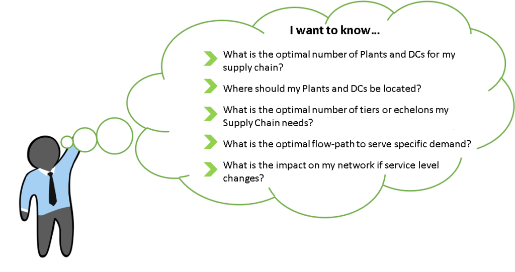
Question: Given these demand points where should be my production plants be located?
We want to know where should we open our plants so that these demand locations are optimally served? What should be the location(s) if I were to open only 1 plant? 2 plants? 3 plants? 4 plants?
Approach
The first step towards a “good” network is to have a clear and accurate blue print of your customer demand. It is important to understand who the real customers are and what is the real demand. Clean your data for any bull-whip signals or cyclicity.
Second step is to aggregate the demand at a logical level. While designing a country-spanning supply chain network, a reasonable demand aggregation could be city. Theoretically, we can of course model at the most granular level i.e. store or street, but it will require a significantly higher effort in data collection and modelling without much gain in the quality of the results.
Our demand data is already aggregated at the city level.
Third, on this cleaned and aggregated demand data we apply a technique called Centre of Gravity or CoG. As the name suggests, it basically means identifying a “middle point” of demand locations. It is intuitive too - we tend to live in places that are at the “centre” of offices, schools, shopping centres, hospitals etc. This is the same principal at work here.
For mathematically inclined – we want to select plant location(s) such that sum of distances from those location(s) to the demand points is minimal.
We did some Excel magic and voila! We have our COG locations –
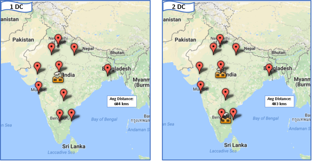
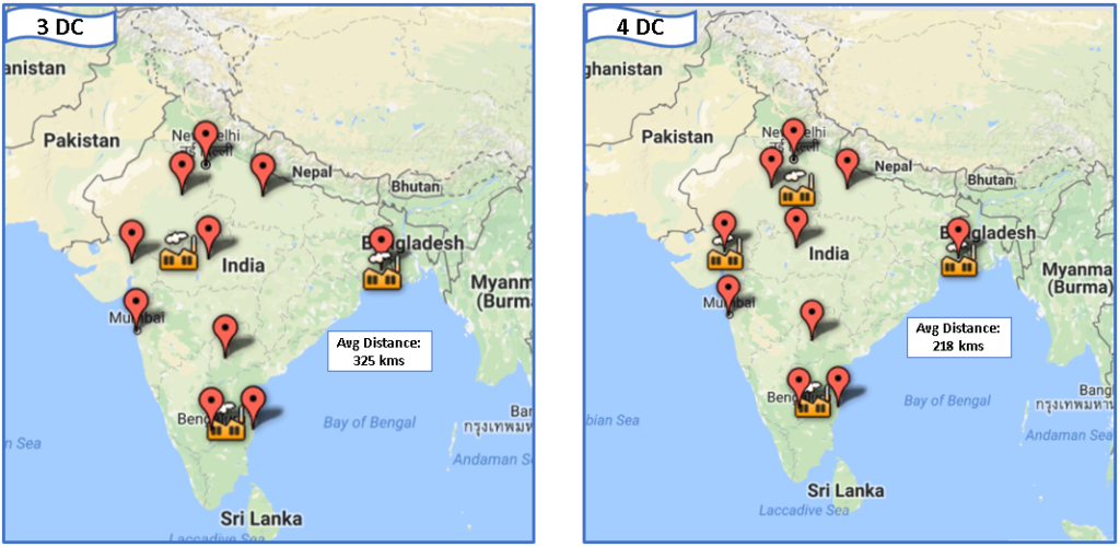
Notice how the average distance decreases as we open more plants. If we open just one plant, the average distance to customer is 684 kms but if we open four, the average distance reduces to 218 kms. Assuming transportation costs to be proportional to the distance for this specific case, then adding three DCs to the network reduces the transportation costs by 68% !
Excel Modelling
So how did we arrive at those precise Centre of Gravity locations? The answer: Excel Modeling. We asked the excel solver to tell us COG locations so that the total distance between the COG location (plant) and demand is minimized. Download the Greenfield Solver here.
If you are new to Optimization and Excel Solver, I strongly recommend you to check out our previous article on this topic before reading further. Done? Good. Now let’s see how we modeled this problem in solver to give us COG locations.
1. Decision Variables
We have two key decision variables here
a. Location of plants: Latitude and longitude of the plants
b. Plant to demand mapping: Which plant should serve which DC
2. Objective function
Minimize the total weighted distance from factory to the demand point.
In other words: Minimize Σ (Demand at a region x Distance from COG)
3. Constraints
a. Number of Plants should be equal to as desired by the user
b. Demand points should be served by exactly one plant
c. Latitude variable can vary between -90 deg. and +90 deg.
d. Longitude variable can vary between -180 deg. and +180 deg.
Feel free to play around with the model. However, be warned that due to non-linear nature of the problem, solver takes a long time to solve particularly for 4-COG model. For reference, it took 30 mins to solve for 4-COG model at moderate tolerance settings. (i.e. we asked solver to give us a “good” solution rather than a perfect one which would take even longer to solve.)
It will be quite difficult to solve a 5 or more COG model without moving to more advanced solver engines or tools. There are many advanced tools in the market that are highly recommended for thorough network strategy projects. We will look at some of these tools in the later articles in the same series.
Conclusion
COG is used in various ways – apart from getting potential locations from scratch, you can also use it to compare the efficiency of your existing network. For e.g., let’s say that we had an existing network of 4 DCs for the demand locations that we just saw now, but at different locations than what greenfield recommended. And if we know that the average distance in that network is 400 kms then we can state that we traveling an extra 180 kms to service the same demand! Against 220 kms that an ideal network delivers. And this inefficiency translates into additional costs and lower service levels.
So, now we have got four answers for the COG problem. We know where we would put our plants if we were to open 1,2,3 or 4 plants. But then the next big question arises - What is the correct number of plants? Should I open four small plants across the country or just a big one at the centre? Or something in between?
Don’t worry – your SCD journey to become a Ninja level Network Strategy Expert has just begun. Keep tuned in for the next article in series and subscribe to our blog to get notified.
Was this article useful? Let us know through your comments.
How long should Excel run before it finds the answer of 4 cog in your model?
Hi Eugenie, 4 COG took about 10-15 mins. This is a NP Hard problem so we expect the time taken to increase exponentially with number of COGs.