Computational Geometry-Based Surface Reconstruction for Volume Estimation: A Case Study on Magnitude-Frequency Relations for a LiDAR-Derived Rockfall Inventory

Abstract

Key to the quantification of rockfall hazard is an understanding of its magnitude-frequency behaviour. Remote sensing has allowed for the accurate observation of rockfall activity, with methods being developed for digitally assembling the monitored occurrences into a rockfall database. A prevalent challenge is the quantification of rockfall volume, whilst fully considering the 3D information stored in each of the extracted rockfall point clouds. Surface reconstruction is utilized to construct a 3D digital surface representation, allowing for an estimation of the volume of space that a point cloud occupies. Given various point cloud imperfections, it is difficult for methods to generate digital surface representations of rockfall with detailed geometry and correct topology. In this study, we tested four different computational geometry-based surface reconstruction methods on a database comprised of 3668 rockfalls. The database was derived from a 5-year LiDAR monitoring campaign of an active rock slope in interior British Columbia, Canada. Each method resulted in a different magnitude-frequency distribution of rockfall. The implications of 3D volume estimation were demonstrated utilizing surface mesh visualization, cumulative magnitude-frequency plots, power-law fitting, and projected annual frequencies of rockfall occurrence. The 3D volume estimation methods caused a notable shift in the magnitude-frequency relations, while the power-law scaling parameters remained relatively similar. We determined that the optimal 3D volume calculation approach is a hybrid methodology comprised of the Power Crust reconstruction and the Alpha Solid reconstruction. The Alpha Solid approach is to be used on small-scale point clouds, characterized with high curvatures relative to their sampling density, which challenge the Power Crust sampling assumptions.

1. Introduction

1.1. Rockfall Hazard

Landslides are defined as mass movements of geological materials downslope [1], and are further classified by their failure mechanisms, geotechnical material, and propagation dynamics [2]. Rugged mountainous terrain around the world is often the source of substantial landslide hazards, particularly related to rock slope instability, where rockfall represents the lower magnitude of rock slope failures. Rockfall is characterized as discrete fragment(s) of rock which detach from a cliff face and, subsequently, fall, bounce, and roll as the fragment(s) propagate downslope as individual rigid bodies [2]. Rockfall is a challenge to manage in mountainous regions, because occurrences can exert large amounts of kinetic energy on impact and may be frequently distributed throughout the area [3]. Quantitative hazard and risk assessment frameworks are utilized to understand and manage rockfall hazard, where an understanding of the magnitude-frequency behaviour of rockfall is required [4,5,6,7]. As part of these assessments, the development of rockfall magnitude-frequency relations has therefore become a common procedure, in which an inventory of known events across a sufficiently long time interval is used to derive the relation across a corresponding spatial domain [8].

Over decades of research, it has been noted that rockfalls exhibit a magnitude-frequency behaviour which can be described by a power law across a range of magnitudes [8]. The power law probability distribution is given by the following probability density function (PDF):

$$P\left(x\right)= C{x}^{-b}$$

(1)

where $b$ is the scaling parameter, $x$ is the observed value (i.e., rockfall magnitude), and $C$ is the normalization constant. At lower magnitudes, a rollover effect in the magnitude-frequency relation of landslides has been noted, where the power-law relation no longer describes the relation [9,10]. The PDF diverges as $x\to 0$ and thus requires a lower bound $x_{min}> 0$. It is therefore said that the ‘tail’ of a distribution follows a power law [11]. For normalization to hold true, the distributions must have $b>1$, thus the PDF is given by:

$$P\left(x\right)= \frac{b-1}{x_{min}} {\left(\frac{x}{x_{min}}\right)}^{-b}$$

(2)

Research surrounding landslides have considered that the rollover effect may be a result of the physical and mechanical characteristics of landslides, in addition to data censoring [10,12,13,14,15]. As such, numerous power-law-based distribution models which consider the rollover effect have been utilized to represent the magnitude-frequency relation of landslides [9,10,16,17].

For rockfall hazards, the magnitude-frequency rollover is thought to be caused solely by censoring [9]. This censoring is attributed to the underreporting of rockfall events, the obscuring of physical rockfall evidence, or the lack of a sufficiently long time interval needed to capture a true measurement of rockfall activity [7]. Rockfall magnitude-frequency is therefore commonly represented by a power law relation which utilizes a minimum magnitude cut-off where the rollover occurs [7,18]. Corominas et al. [8] suggest that there should also be an upper bound truncation on the magnitude-frequency relation with regard to a maximum credible event, where the magnitude should be defined considering the geostructural and geomechanical setting.

1.2. Rockfall Magnitude-Frequency Relations in the Digital Age

To derive magnitude-frequency relationships, landslide inventories are traditionally created by actively documenting recent occurrences, gathering relevant historical data, and by conducting field mapping. In appropriate environments, dendrogeomorphological investigations may be feasible as well to investigate historical occurrences [19]. Over the past few decades, the development of remote sensing platforms for capturing highly detailed spatial data of the surface environment, in addition to the parallel evolution of modern computer hardware and software, has provided a means for landslide inventories to be built digitally, by monitoring changes in the terrain through a comparison of spatial data acquired over a time interval [18,20,21,22,23,24].

To detect rockfall, light detection and ranging (LiDAR) or photogrammetry surveys are deployed in terrestrial and oblique configurations in order to collect information of the steep source areas [25]. Recently, a helicopter mounted mobile LiDAR system has been used to increase the extents of rockfall monitoring to a 20 km length of coastal cliffs in England [26], and the development of several automated acquisition and processing workflows have supported the increased frequency of rockfall monitoring [18,27,28,29]. Table 1 summarizes several monitoring methodologies, which operated on sequential LiDAR datasets, to extract and measure the volume of rockfalls. On the next few pages, we briefly describe the key components of a rockfall extraction workflow, and introduce the challenges associated with accurately estimating the volume of the detected rockfalls.

LiDAR and photogrammetry are used in many fields outside of landslide hazards as well. Telling et al. [30] provide a review of applications of terrestrial laser scanning (TLS) applications in the geosciences and the application of TLS for monitoring rock slope instabilities is reviewed by to Abellán et al. [31]. Readers are referred to Smith et al. [32] and Anderson et al. [33] for reviews on the use of structure from motion multi-view stereo photogrammetry in the geosciences.

Table 1. Summary of several recent rockfall extraction methodologies, ordered by the most recent publications. Some methods additionally conduct post-database filtering by the point cloud volumes, number of points, or the change detection signature. Site dimensions preceded with a tilde indicate approximate measurements made when the dimensions were not explicitly stated in the text. Data acquisition frequencies were taken as median, or as fact from the texts.

Study	Timespan [Years]	Median Frequency	Site Dimensions	Change Detection Method	Clutter Removal	Clustering	Volume
Guerin et al. [34]	11	365 days	~160 × 600 m	C2M 1	Neighbour averaging	DBSCAN	SfR 2: Manually w/3D software
Hartmeyer et al. [35]	6	yearly	5-rockwalls: 234,700 m2	M3C2 3	-	Region growing	Sum of raster cells
DiFrancesco et al. [36]	5.0	69 days	240 × 120 m	M3C2	Manual	DBSCAN 4	SfR: Alpha Solid
Benjamin et al. [26]	2.6	309 days	20.5 km × (30–150 m)	M3C2	Manual	DBSCAN	SfR: Power Crust
Guerin et al. [37]	40	34 years–1 month	~0.8 × 0.6 km; ~1.5 × 0.8 km; ~1.8 × 0.8 km;	C2M	Neighbour averaging	DBSCAN	SfR: Manually w/3D software
Williams et al. [18,38]	0.8	1 h–30 days	210 × 60 m	M3C2 (variable search lengths)	Waveform + edge filter; Noise mask	Region growing	Sum of raster cells
Van Veen et al. [39]	1.3	76 days	1.1 km × 500 m	M3C2 (nearest neighbors)	-	DBSCAN	SfR: Alpha Shapes *
Olsen et al. [40]	1.8	11 months	340 × 170 m; 110 × 11 m; 90 × 8 m	DoD 5	Raster averaging	Region growing	Sum of triangulated raster cells
Carrea et al. [41]	3.0	6 months	~80 × 40 m	C2M	-	DBSCAN	SfR: Alpha Shapes *

¹ Cloud-to-model comparison [42]. Computes the distance from each point to a neighbouring triangular mesh facet, along the facet normal. ² Surface reconstruction for three-dimensional volume estimation. ³ Multiscale model-to-model cloud comparison [43]. Computes locally averaged change between two-point clouds along a locally oriented surface normal. ⁴ Density-based spatial clustering of applications with noise [44]. Clusters data considering a minimum number of points within a minimum search radius. ⁵ Difference of digital elevation models (DEMs). Computes change between rasters, orthogonal to the raster image orientation. * Surface reconstruction mesh hole filling method not specified and/or provided.

Table 1. Summary of several recent rockfall extraction methodologies, ordered by the most recent publications. Some methods additionally conduct post-database filtering by the point cloud volumes, number of points, or the change detection signature. Site dimensions preceded with a tilde indicate approximate measurements made when the dimensions were not explicitly stated in the text. Data acquisition frequencies were taken as median, or as fact from the texts.

Study	Timespan [Years]	Median Frequency	Site Dimensions	Change Detection Method	Clutter Removal	Clustering	Volume
Guerin et al. [34]	11	365 days	~160 × 600 m	C2M 1	Neighbour averaging	DBSCAN	SfR 2: Manually w/3D software
Hartmeyer et al. [35]	6	yearly	5-rockwalls: 234,700 m2	M3C2 3	-	Region growing	Sum of raster cells
DiFrancesco et al. [36]	5.0	69 days	240 × 120 m	M3C2	Manual	DBSCAN 4	SfR: Alpha Solid
Benjamin et al. [26]	2.6	309 days	20.5 km × (30–150 m)	M3C2	Manual	DBSCAN	SfR: Power Crust
Guerin et al. [37]	40	34 years–1 month	~0.8 × 0.6 km; ~1.5 × 0.8 km; ~1.8 × 0.8 km;	C2M	Neighbour averaging	DBSCAN	SfR: Manually w/3D software
Williams et al. [18,38]	0.8	1 h–30 days	210 × 60 m	M3C2 (variable search lengths)	Waveform + edge filter; Noise mask	Region growing	Sum of raster cells
Van Veen et al. [39]	1.3	76 days	1.1 km × 500 m	M3C2 (nearest neighbors)	-	DBSCAN	SfR: Alpha Shapes *
Olsen et al. [40]	1.8	11 months	340 × 170 m; 110 × 11 m; 90 × 8 m	DoD 5	Raster averaging	Region growing	Sum of triangulated raster cells
Carrea et al. [41]	3.0	6 months	~80 × 40 m	C2M	-	DBSCAN	SfR: Alpha Shapes *

¹ Cloud-to-model comparison [42]. Computes the distance from each point to a neighbouring triangular mesh facet, along the facet normal. ² Surface reconstruction for three-dimensional volume estimation. ³ Multiscale model-to-model cloud comparison [43]. Computes locally averaged change between two-point clouds along a locally oriented surface normal. ⁴ Density-based spatial clustering of applications with noise [44]. Clusters data considering a minimum number of points within a minimum search radius. ⁵ Difference of digital elevation models (DEMs). Computes change between rasters, orthogonal to the raster image orientation. * Surface reconstruction mesh hole filling method not specified and/or provided.

The detailed spatial information captured by LiDAR and photogrammetry is stored within a point cloud, a collection of points in 3-dimensional (3D) space. Each point cloud provides a permanent digital record of the terrain visible by the survey at a particular instance in time, while their spatial coverage is limited by the survey view. Changes in the terrain over time can be identified by computing distances between co-registered point clouds, in a process called change detection. Conducting change detection on the sequential clouds twice—treating both clouds as the reference, allows for the identification of the backs and fronts of the changing features captured within the point cloud [45]. The changing features can be extracted from the change detection results by extracting significant changes with respect to a limit of detection, and merging the backs and fronts into a singular cloud. The limit of detection typically determined as a function of the global registration error, and can be spatially varied considering local point cloud roughness [43]. Extracting rockfall from the significant change requires (1) classifying the detected areas of loss corresponding to rockfall, (2) removing noise and artifacts in the change detection signature, and (3) clustering the filtered changes into individual point cloud subsets corresponding to discrete 3D rockfall events. All portions of the semi-automated processing workflow can have a substantial impact its efficiency, accuracy, and robustness.

Measurement of failed rockfall volume is critical in the development of a magnitude-frequency relation. To determine rockfall volume in 3D, a representative digital surface must be reconstructed from the extracted point cloud. This task is addressed by the field of surface reconstruction, in which the goal is to recover an accurate digital representation of a physical object that has been scanned from the real world [46]. There is an inherent difficulty in doing so for our application, considering the desired reconstruction accuracy, versus the existence of various point cloud imperfections, as we note in Section 1.3.

To simplify the issue of computing rockfall volumes in 3D, numerous workflows have projected the rockfall point clouds into 2.5D raster datasets and computed the volumes as a summation of the grid cells multiplied by their change value (Table 1). However, Benjamin et al. [47] showed that raster-based volume calculations result in high volumetric errors. These computations are sensitive to the projection method and orientation as well as the cell size. Geometrically challenging terrains, with large variations of surface orientations and overhanging features, are not captured well by 2.5D rasters. Therefore, there are merits in assembling digital rockfall inventories with fully 3D methods.

1.3. Surface Reconstruction Challenges and Requirements

As introduced earlier, to compute the volume of a point cloud in 3D, a representative surface must be reconstructed, from which the volume can be estimated. Berger et al. [48] review the state-of-the-art methods in surface reconstruction. The authors note that the overarching challenge within the field of surface reconstruction is to recover an accurate digital surface representation of an object, given a point cloud input with imperfections summarized in Figure 1.

Evidently, not all resulting point clouds from a semi-automated rockfall extraction will be perfect candidates for surface reconstruction applications; this is a result of the site geometry relative to the survey setup, instrumental error, human error during the data processing pipeline, environmental factors such as lighting for photogrammetry, or atmospheric and surface moisture for LiDAR, as well as potential systematic errors within the semi-automated rockfall extraction.

Our utilization of surface reconstruction, therefore, requires methods to be robust in dealing with these various point cloud imperfections. Further, the methods must produce surfaces with correct topology and global geometry, leading to a correct estimation of volume. It should be noted that local errors in the surface representation can accumulate to cause an incorrect rockfall volume. Therefore, a good surface reconstruction method should be able to reconstruct the correct topology considering the presence of point cloud imperfections, while also capturing the local surface details.

Given that we are concerned with reconstructing the surface of real world scanned rockfalls, there are a few topological requirements for our reconstructed surface: (1) the surface must be fully enclosed (i.e., watertight), and (2) the surface must be topologically equivalent to 3D objects in the real world. These requirements are encapsulated by the definition of a 2-dimensional manifold, or 2-manifold (Figure 2). A manifold is a topological space, where locally, subsets are homeomorphic to the Euclidean space of the equivalent topological dimension [49]. For a 2-manifold, this concept of homeomorphism means that local portions of the surface can be continuously deformed onto a 2D Euclidean disk without requiring cutting, gluing, or self intersection. An example of a 2-manifold is a sphere. A sphere is homeomorphic to an open disk when we evaluate it at local sections; however globally, it is not.

There are two further requirements for surfaces to be topologically equivalent to the solid rockfall objects. Firstly, the 2-manifold must be orientable, meaning it has consistent orientation; traversing along the surface should not allow one to mirror onto the other side of the surface. Secondly, the 2-manifold should be free of self-intersections when realized in 3D Euclidean space. In topology, the “Klein bottle” is a well-known exemplification of a 2-manfold which does not fulfill these two criteria.

1.4. Digital Surface Representation and Reconstruction Methods Background

Surface reconstruction methods produce either implicit or explicit digital surface representations [51]. Implicit surface representations define a surface as a particular isocontour of a scalar function [51], such as the zero-value of the signed distance function [46], or an isovalue of the indicator function which approximates the surface boundary [52]. Triangulated meshes can then be extracted from the implicit functions utilizing volumetric methods, such as the Marching Cubes algorithm [53]. Implicit surface reconstruction methods typically require an estimate of the oriented point cloud normals, however, determining consistent orientation across the point cloud is a difficult task with the presence of point cloud imperfections [48]. Some methods may treat randomly distributed incorrect orientations as noise, although most methods struggle when encountering clusters of incorrect normal orientations [48]. Another difficulty is that point cloud imperfections make it difficult to determine an appropriate scale used to estimate the point normal vectors [43,46]. Some surface reconstruction methods have utilized additional point cloud information, such as scanner or camera positions, to achieve correct point normal orientations.

Explicit surface representations precisely define a surface as (1) a single parametric function, or (2) a set of surface patches allowed to show curvature, such as Non-Uniform Rational Basis-Splines (NURBS), or (3) a discrete surface tiled by flat surface patches, such as a discrete polyhedron. The much higher complexity of geometric operations on continuous curved surfaces resulted in a preference towards the discrete representation of explicit surfaces utilizing discrete polyhedrons, such as triangulated meshes. Discrete polyhedrons allow for the fast robust implementation of geometric operations, which are well suited for rapid processing on a graphics processing unit (GPU). Explicit surface reconstruction methods have therefore focussed on establishing topological connections within the point cloud, as a subset of its Delaunay Triangulation, and relying on computational geometry to do so [54,55,56,57].

The computational geometry based explicit surface reconstruction methods have been adopted for several of the examples of semi-automated rockfall extraction and volume computation workflows as shown in Table 1. These methods are more desirable for our application because the discrete surfaces, determined via computational geometry, directly honour the input data points, while the continuous surface representations might not. Additionally, the requirement for accurate normal vectors with correct orientations adds a degree of complexity into the implicit surface reconstruction methods, which makes them less desirable to incorporate within the automated rockfall database systems. In this study, we therefore exclusively focus on the discrete polyhedral surface representations determined via computational geometry.

1.5. Study Objectives

In a short case study utilizing a synthetic test object and three real rockfall events, Bonneau et al. [50] determined that computational geometry-based surface reconstruction methods include explicit biases, which can cause substantial error on the rockfall volumes calculated. The presented article aims to further the study of Bonneau et al., by investigating the influence of volumetric error across a magnitude-frequency relation. This endeavour requires a much larger scale of analysis, with a high number of rockfall events across varying orders of magnitude. We therefore investigate four surface reconstruction techniques on a high quality digital rockfall database derived from 5-years of terrestrial laser scanning monitoring at an active rock slope in southwestern British Columbia (BC), Canada, using the digital rockfall database from DiFrancesco et al. [36]. This database contains 3668 rockfall point clouds ranging from 12-points to nearly 100,000-points.

In this study, we summarize four computational geometry surface reconstruction methods and cover the fundamental tools used in their process. We present a technique to automate the Power Crust surface reconstruction method developed by Amenta et al. [55], and devise a method to deal with erroneous outputs. We evaluate the results of applying each surface reconstruction technique to the 5-year long digital rockfall database. We discuss the results using rank-frequency cumulative distribution plots, maximum likelihood estimation of power law parameters, and projected annual frequencies computed with the power-law models. We discuss the trends and provide visual examples of reconstructed 3D meshes to support the observations. To conclude, we make recommendations for the future usage of these methods in determining the volume of digital objects described by point clouds.

2. Materials and Methods

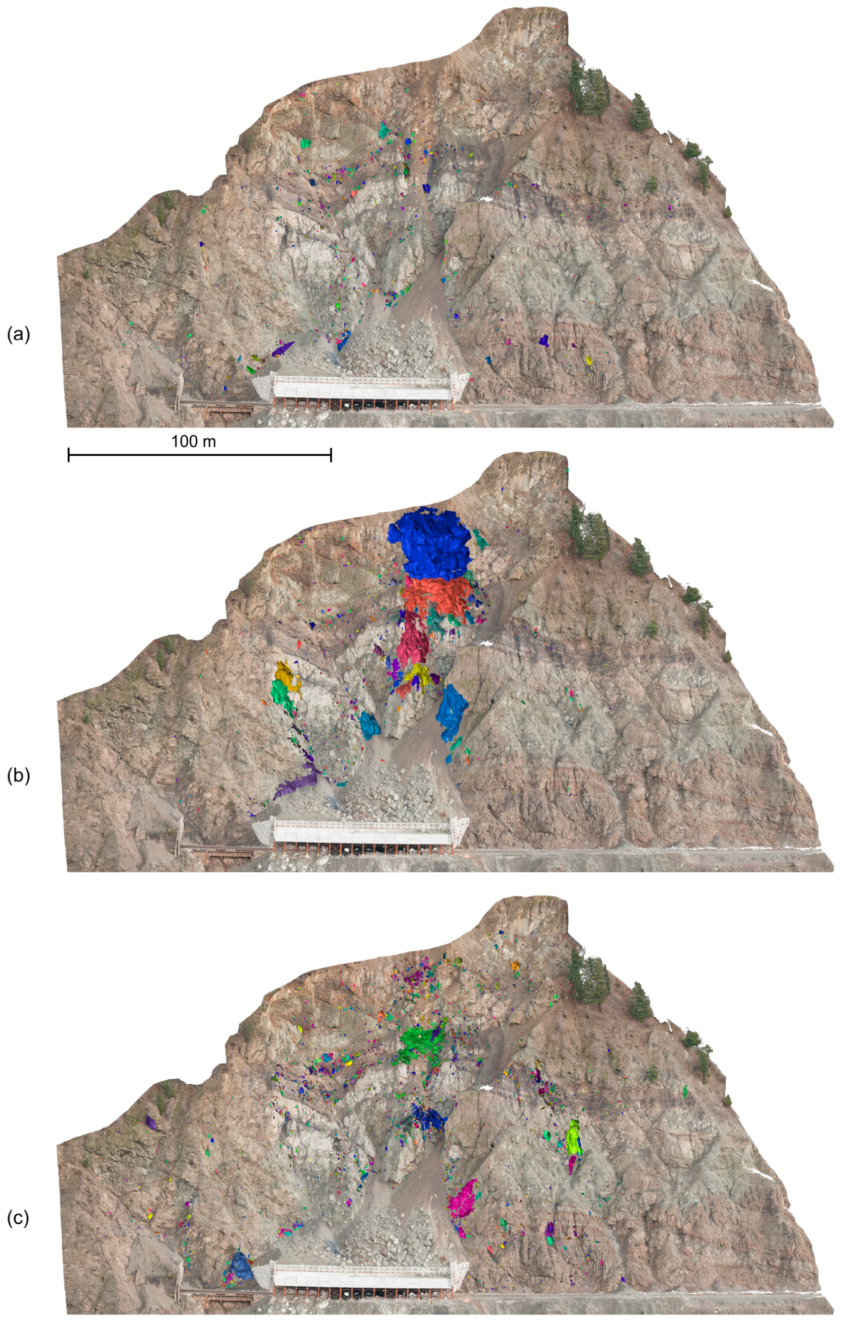
2.1. LiDAR-Derived 3D Rockfall Database

This study utilized the 5-year long rockfall inventory presented by DiFrancesco et al. [36], derived from 27 sets of TLS data acquisitions captured at weekly to seasonal frequencies from November 2013 to December 2018. Figure 3 on the following page shows the 5-year rockfall monitoring conducted at the study site, across three selected time intervals for enhanced visualization. Each individual rockfall extracted is colourized differently and projected onto a photogrammetry model for visualization.

The study site is an active engineered rock slope, located adjacent to the Canadian National rail line, which runs along the Fraser River in Interior British Columbia, Canada. The bedrock consists of a succession of Cretaceous deltaic sedimentary rocks [58]. Local scale faulting has been identified as a key factor for contributing to the relatively high activity of rock slope failures seen early in the 2010’s, which sparked interest in monitoring the site [25,59,60].

The TLS datasets were captured with an Optech Ilris 3D time-of-flight system (20 datasets; November 2013–September 2017), and a Riegl VZ-400i time-of-flight system (7 datasets; September 2017–December 2018). The Optech system has a manufacturer-specified accuracy of 7 mm in range and 8 mm in vertical and horizontal directions from a distance of 100 m [61]. The Optech system has a maximum range of approximately 800 m at 20% target reflectivity [62]. The Riegl system has a manufacturer-specified accuracy of 5 mm and precision of 3 mm from a distance of 100 m [63]. The Riegl system has a maximum range of approximately 400 m at 20% reflectivity with a 100 Hz pulse rate [63]. Scans were taken from a vantage point approximately 400 to 500 m away from the slope. Vertical extents ranged from 130 to 170 m and horizontal extents ranged from 200 to 300 m. The typical registration error ranged between 1–2 cm, and a conservative limit of detection of 5 cm was utilized in extracting rockfall. The extracted change corresponding to rockfall was subsampled to a point spacing of 10 cm.

The rockfall database used in the present study was one of six created, as part of a parametric analysis evaluating semi-automated rockfall extraction. DiFrancesco et al. [36] considered the impact of the spatial averaging component of a widely used point cloud-based change detection algorithm (multiscale model-to-model cloud comparison, or M3C2). The database used in the current study is the most detailed database generated from the study, and contains 3668 rockfalls.

The numerous stages in the semi-automated rockfall extraction workflow briefly discussed in Section 1.2 greatly influence the resulting rockfall database [36]. For brevity, the volume computation component is the sole focus of this study. In the presented study, the authors, therefore, work with a collection of discrete rockfall point clouds which have already been detected and manually verified. Readers are referred to DiFrancesco et al. [36] for a detailed overview of the study site, survey, data processing, and the rockfall extraction workflow used. The studies in Table 1 provide examples of other semi-automated rockfall extraction methodologies.

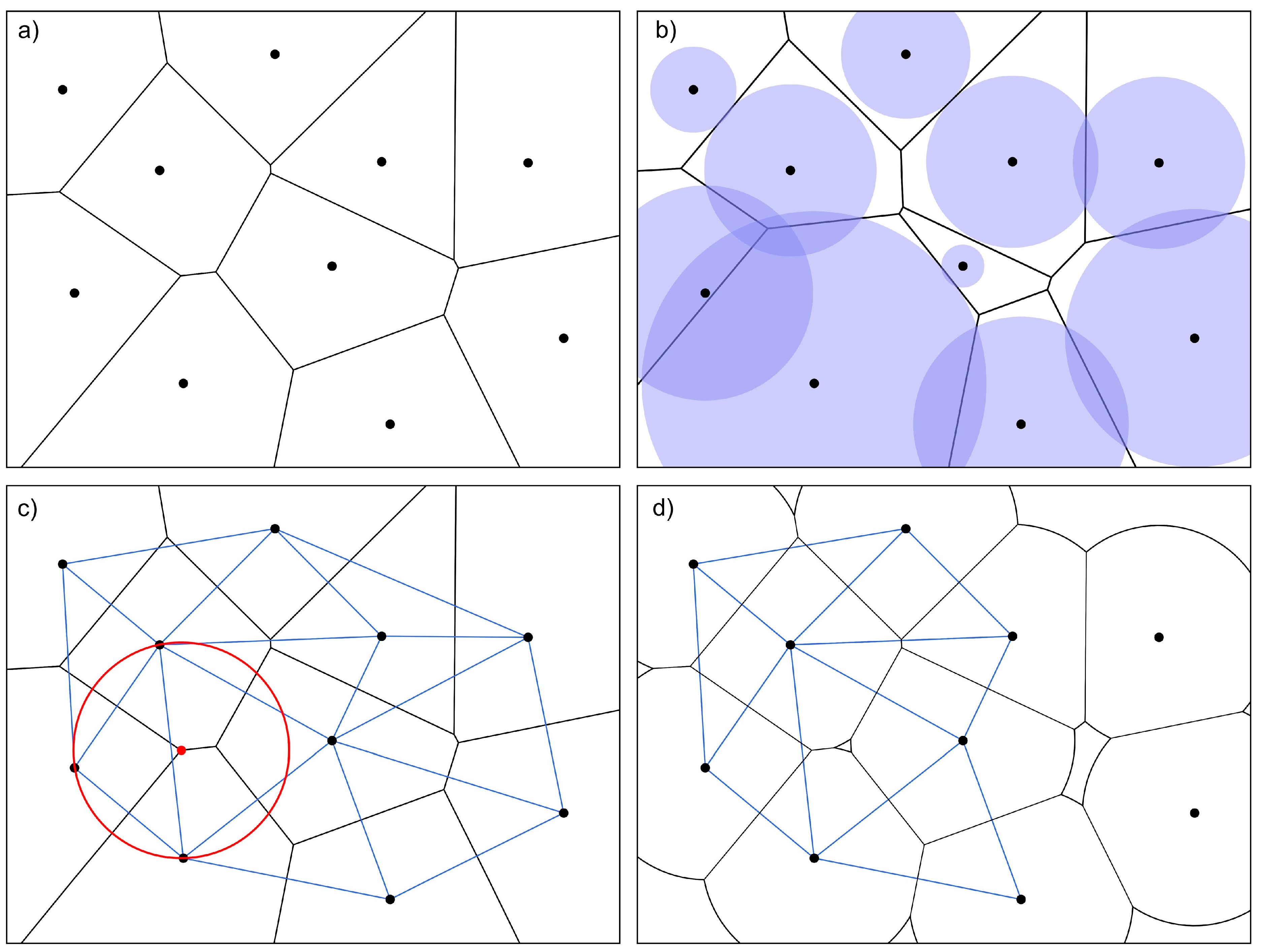
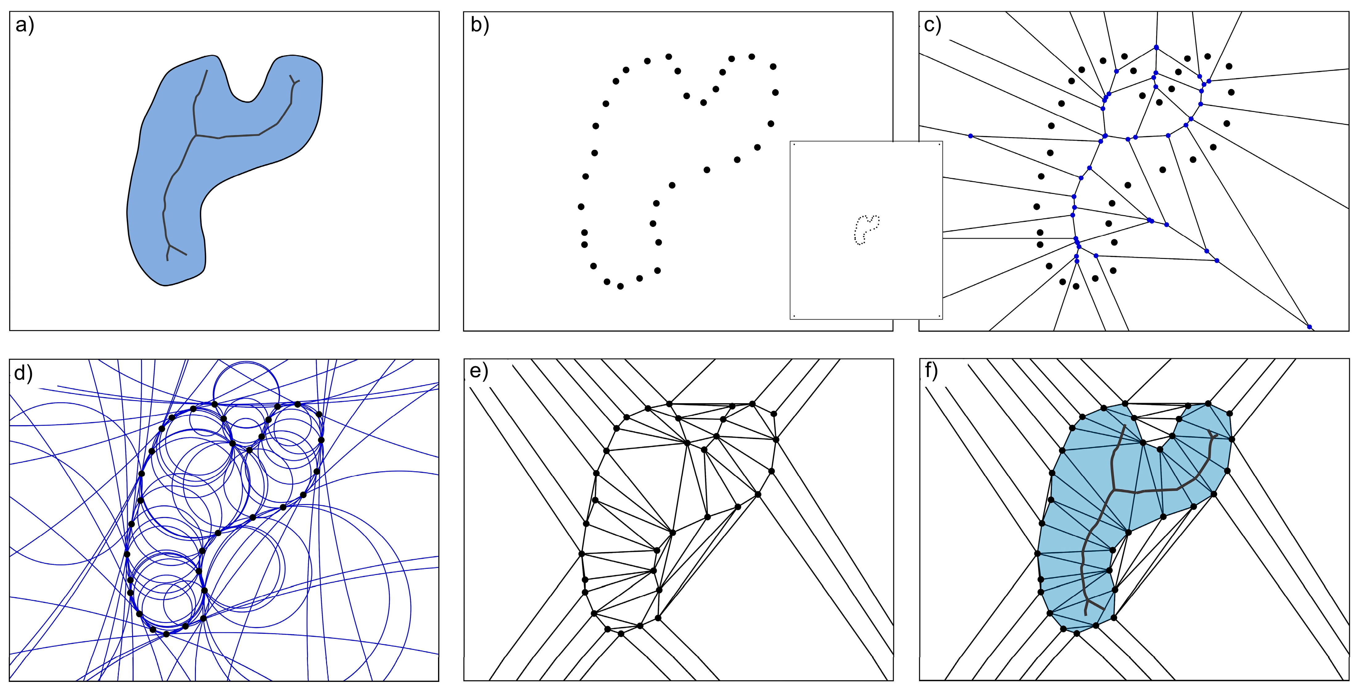
2.2. Computational Geometry Tools

Computational geometry methodologies are more than often presented in mathematical notation, as lemmas and algorithms, rather than in a qualitative and graphical manner suitable for wider audiences. There are several computational geometry concepts that form the basis for understanding the more complex surface reconstruction algorithms—which are the main focus of this article. This section provides general descriptions of several fundamental structures of computational geometry. These structures are the Voronoi Diagram and its dual graph, the Delaunay Triangulation. The 3D explanations of these concepts transfer appropriately into 2D and are visualized in Figure 4 to aid our definitions. Note that all proximity and distance metrics utilized in the definitions refer to Euclidean distance.

The first concept is the Voronoi Diagram. A 3D Voronoi cell is a 3D space which contains all space most proximal to its sample point. A 3D Voronoi cell is bounded by a series of planes. A Voronoi diagram is the collection of these Voronoi cells (see Figure 4a). The second concept is a variant of the Voronoi Diagram, called a Power Diagram. A 3D Power cell incorporates weights for each of the sample points. The 3D Power cell contains all 3D space, in which the Power distance (the distance subtracted by its weight) is less than the Power distance of competing cells (see Figure 4b). The last variant of the Voronoi diagram does not have a formal name. We refer to it as the “restricted Voronoi diagram”. Similarly, each restricted Voronoi cell contains its most proximal space. However, a uniform weight (i.e., distance) is used to limit the maximum span of all cells (see Figure 4d).

The Delaunay Triangulation is closely related to the Voronoi diagram. A 3D Delaunay Triangulation is built with tetrahedra, which encompass corresponding triangles, edges, and points. A Delaunay tetrahedron is defined from an empty circumsphere, which intersects four sample points along its boundary, without containing any sample points inside of it (see an empty circumcircle plotted in red in Figure 4c).

A Delaunay tetrahedron can be drawn by connecting the samples corresponding to 4-adjoining Voronoi cells. Similarly, in 2D, triangles are connected by 3-adjoining 2D Voronoi cells. This is the dual-graph relationship between the Voronoi Diagram and its Delaunay Triangulation, and is illustrated in Figure 4c,d. Note that the restricted Voronoi diagram in Figure 4d changes the cell adjacencies, and therefore results in a different triangulation; this is also called an Alpha Complex [49], which we discuss further in the next subsection.

Readers are referred to Edelsbrunner [68] for a thorough definition of the Voronoi Diagram and its dual Delaunay Triangulation in 2D, as they relate to the fundamental concepts and algorithms of computational geometry.

2.3. Computational Geometry Surface Reconstruction for Volume Estimation

With knowledge of some of the fundamental computational geometry concepts, we now set to describe each of the 3D surface reconstruction methods with the aid of 2D graphical descriptions. We hope that readers will understand the underlying assumptions that each method makes, as they relate to the errors that are realized in estimating the volumes of the LiDAR-derived rockfall database.

2.3.1. Convex Hull

The Convex Hull is a fundamental concept of topology and computational geometry, and is used throughout numerous fields. The Convex Hull of a set of points, S, is the smallest convex set that contains it, which is the set of all convex combinations containing S [49]. The convex hull of a 3D point set thus results in the smallest convex polyhedron encompassing all points (Figure 5i). The Convex Hull reconstruction was implemented using the tetrahedron-based Alpha Shape implementation in Matlab [69], utilizing an infinite Alpha Radius (see next subsection). Computing the volume of the tetrahedron-based shape representations simply requires the summing of the tetrahedron volumes, which was also carried out in Matlab.

2.3.2. Three Dimensional Alpha Shapes

Edelsbrunner and Mücke [56] formally defined the three-dimensional Alpha Shape of a point set as the union of simplices covered by all Delaunay tetrahedra having empty circumspheres, with radii less than the defined radius—referred to as the Alpha Radius. Simplices are thus the building blocks of the Alpha Shape, with a k-dimensional simplex being the convex hull of $k+1$ affinely independent points [49]. A point, edge, triangle, and tetrahedron, are respectively described by the 0, 1, 2, and 3-simplex.

The value of Alpha Radius prescribes a limiting distance for the extents of all Voronoi cells, and thus determines the connectivity of the Delaunay triangulation. Figure 5 shows the progression of an increase in the Alpha Radius, leading to a change in the resulting Alpha Shape. For a set of points, there therefore exists a family of Alpha Shapes, with each member corresponding to a different value of Alpha Radius. The value of Alpha Radius determines the tetrahedra and encompassing k-dimensional simplices generated by the Delaunay triangulation. The Alpha Radius can range from zero to infinity, where an infinite value results in the convex hull, thus simplifying the surface of the shape (Figure 5i), and a zero-Alpha Radius results in an empty shape, comprised of only 0-simplices (Figure 5a). Therefore, an optimal value of Alpha is required to best approximate the geometry of the object while producing a 2-manifold watertight reconstruction. Lower values of Alpha can capture local shape details while larger values of Alpha can capture the global shape (Figure 5).

Readers are referred to Edelsbrunner and Mücke [56] for further details and discussions of Alpha Shapes. Two variations of the Alpha Shape algorithm are utilized in this study, both of which were implemented in Matlab. The Alpha Shape volumes were computed by summing the volume of the tetrahedra in Matlab.

The first method is the Default Alpha Shape, which has an Alpha Radius such that all points are utilized in the Delaunay Triangulation—referred to as the Default Alpha Radius. The exterior boundary of the Default Alpha Shape, defined by triangular facets, is therefore not guaranteed to be 2-manifold and watertight.

The second variation is the Alpha Solid method, which iterates through the family of Alpha Shapes, and determines the smallest value of Alpha that produces a mesh whose boundary facets are 2-manifold and watertight. This is achieved by ensuring that for each edge $p_1{p}_2$ there exists the edge $p_2{p}_1$ corresponding to the shared edge with an adjacent face, which we refer to as the “half-edge criteria”. The family of unique Alpha Shapes is given by the Alpha Spectrum, which is the set of all unique values of Alpha, corresponding to all possible $k$-simplices with empty circumspheres for $1\le k \le 3$. We follow the method of Bernardini et al. [70] to reduce the computation time, by bisecting the Alpha Spectrum list to find the lowest value of Alpha. In this process, we only consider Alpha Radii which include all input points (i.e., radii larger than the Default Alpha Radius). A previous implementation of this method without bisection was presented by Bonneau et al. [50] as the “iterative Alpha-shape” approach.

In our tests implemented in MATLAB, there was no critical level of Alpha, above which all resulting Alpha Shapes fit the half-edge criteria. We found that alternating chunks of the Alpha Spectrum had instances of an edge repeated 4 times, thus not satisfying the half-edge criteria. To overcome this issue, we bisect the Alpha Spectrum to find the lowest Alpha Radius with only one instance of 4 repeated edges. Then, we ascend the Alpha Spectrum list from this position to find the lowest Alpha Radius which satisfies the half-edge criteria. We compared the results to those achieved by ascending the Alpha Spectrum list without bisecting, and confirm that the results agree with each other. This results in a fast, robust implementation that guarantees a 2-manifold and watertight Alpha Shape.

2.3.3. Power Crust

The last surface reconstruction method we investigate also computes the surface as a subset of the Delaunay Triangulation, and utilizes interesting properties of the object’s shape related to the Voronoi Diagram of its point set. The Power Crust algorithm created by Amenta et al. [55], takes the sample of points and constructs a piecewise-linear approximation of the object’s surface, as a polygonal surface mesh, which is guaranteed to be watertight. Several concepts must be defined, with knowledge of the computational geometry concepts introduced earlier in Section 2.2. These additional tools are illustrated in Figure 6 and are defined below:

• Poles: A subset of the Voronoi vertices, located on the interior and exterior of the object, but not along the object’s surface;
• Polar balls: The balls centered at the poles, each with radii such that they are touching the nearest input point sample;
• Medial axis: The skeleton of a closed shape, along which, points are equidistant to two or more locations along the shape’s boundary.

Filling a shape with maximal balls (i.e., spheres) centered at its medial axis produces a watertight shape which approximates the shape’s geometry. The algorithm builds from this idea in order to construct the Power Crust. Conceptually, the algorithm approximates the medial axis, and then fills the interior and exterior of the object with maximal balls. The Power Crust is the piecewise-linear surface constructed at the point where the interior and exterior maximal balls intersect (Figure 6).

The Power Diagram is a key tool utilized in determining the Power Crust. The Power Diagram is constructed using the location and weights of the polar balls (i.e., Voronoi vertices), rather than the sample points themselves (i.e., the example in Figure 4b). The Power Crust can then be determined from the Power Diagram of the polar balls, at the polygonal boundaries between the interior and exterior Power cells.

The key requirement for the Power Crust algorithm to be successful, is an input point cloud which is sufficiently sampled. The sampling density of points should be inversely proportional to the nearest distance from the surface to the medial axis. A closer distance from the surface to the medial axis corresponds to a higher curvature (i.e., Figure 6a), which thus requires a larger sampling density [55]. An important note follows this—smaller scale rockfalls will have surfaces closer to their medial axis, however, our point spacing is uniform at 10 cm (excluding occlusions). Therefore, small-scale rockfall point clouds will challenge the Power Crust algorithm. Many of the smaller rockfalls cause the algorithm to break down, which we address at the end of the subsection and further analyze throughout the Results and Discussion sections.

The Voronoi diagram of a sufficiently sampled point cloud will be composed of Voronoi cells that are long, skinny, and perpendicular to the surface (Figure 6c). This is due to the proximity of samples along the surface, the lack of samples in the interior of the shape, and the distance from the surface to the medial axis (Figure 6a,c). The medial axis can then be approximated by the Voronoi vertices found at the intersection of the long and skinny Voronoi cells found in the interior of the shape. The Voronoi vertices approximating the medial axis correspond to interior poles. The interior poles converge to the medial axis as the sampling density approaches infinity [54,71].

The main challenge for the Power Crust algorithm occurs when the input point clouds are not well sampled: it is difficult to determine which poles correspond to Voronoi vertices along the medial axis within the interior of the shape, and which poles correspond to the Voronoi vertices on the exterior of the object. This has problematic effects on volume estimation if not properly handled. To deal with this potential ambiguity, the Power Crust algorithm computes the unlabelled poles at Voronoi vertices belonging to the long and skinny Voronoi cells. The algorithm then determines the weights of the polar balls, constructs the Power Diagram, labels the poles as interior or exterior, and then extracts the Power Crust as the boundary separating the interior Power cells from the exterior.

With an overview on how the Power Crust algorithm functions and its main challenge, we now explain in detail the process of the algorithm. Figure 6 outlines the Power Crust in two-dimensions. First, eight points are added to the input point cloud, via a bounding box which is 5-times larger than the minimum bounding box of the sample points—in our 2D example four points are added (Figure 6b). Next, the Voronoi diagram of the point set is constructed. The bounding box vertices create Voronoi vertices sufficiently far away from the sample points, such that they fit the Voronoi cell shape criteria, and will be confidently considered as known outer poles in the future pole labelling process.

Next, two poles are determined for each sample point, with exclusive consideration of Voronoi vertices belonging to the Voronoi cell of the sample point. The first pole is selected such that it is the furthest connected Voronoi vertex found. The second pole is selected such that it is the furthest Voronoi vertex in the opposite direction from the first. With proper sample point clouds, these poles should be on either side of the surface, with one located in the interior of the object near its medial axis.

Next, the Power diagram is constructed for all poles, with the weight of each cell corresponding to the radius of its polar ball. The Power Diagram splits the 3D space into polyhedral cells (Figure 6e). The polygonal faces belonging to the Power Crust are those which separate the interior Power Diagram cells from the exterior cells (Figure 6f), hence the importance of the labelling step.

To label the poles and their corresponding Power Diagram cells as interior or exterior, a graph data structure is constructed. Two poles are connected in the graph, if they correspond to the pair of poles for a particular sample point (i.e., one inner and one outer). Additionally, two poles are connected if their corresponding Power Diagram cells are adjacent, and share a polygonal face. The labeling algorithm then begins, first by labeling the poles which are closest to the bounding box vertices, as there is a high confidence that they are outer poles. The algorithm knows if two adjacent Power diagram cells both belong to outer poles if their polar balls intersect deeply. This is because an outer polar ball is almost entirely contained on the exterior, while an inner polar ball is almost entirely contained in the interior. The intersection of two outer or two inner polar balls is thus deep, while the intersection of an outer and inner polar ball is shallow. Considering the assumptions that (1) each sample point has an inner and outer pole and (2) deep intersections result in the adjacent pole having the same label, the labelling algorithm therefore simply traverses the graph and labels the poles. Note that these assumptions do not hold true if the surface is not sufficiently sampled, and therefore some poles may be incorrectly labelled.

We utilize the Power Crust software provided by Amenta et al. [55] which has been ported to Microsoft Windows by Alhashim [72]. The implementation of Power Crust was built from Ken Clarkson’s Hull [73] with modifications to construct the Power Diagram. Hull utilizes pseudorandom sampling to increase the expected time of incrementally constructing the Voronoi Diagram as the dual to its Delaunay Triangulation [74]. The usage of random sampling can therefore change the order of the graph utilized to label the interior and exterior poles. For point sets which do not meet the sampling assumptions, this potentially changes the labels of ambiguous poles.

We confirm in our experience that the Power Crust algorithm struggles when the sampling assumptions are not met. Small scale rockfall point clouds, which also have 10 cm point spacing, produce Voronoi diagrams with square-like cells. Large relative gaps can also result in a square-shape of Voronoi cell. These cells can cause some of the labelling assumptions to not hold true, causing incorrect pole labels. Considering the graph-propagation method used by the labelling algorithm; incorrect labels can amplify. Further, the volume of the Power Crust can be significantly overestimated if an outer pole is mislabeled as inner.

To combat the issue with mislabeled outer poles, we conduct a bounding box analysis between the resulting mesh versus the input point set. If the ratio of the bounding box dimensions exceeds a value of 1.2, we reject the result and attempt the reconstruction again. Here we utilize the random sampling of Hull to our advantage; while one Power Crust execution could incorrectly label the poles, the following execution might not. We set the maximum number of attempts to a very conservative number of 50. We flag the IDs of the point clouds which cannot be reconstructed by the Power Crust, and discuss the inputs that failed in the Results Section.

The Power Crust software also prescribes parameters corresponding to the sampling assumptions, and the criteria for rejecting poles based on the Voronoi cell shape. The sampling density constant, R, was set to 1, which is more suitable for sparse point cloud inputs with limited noise and no sharp corners [55], often providing a more robust fit [26]. The remainder of parameters were left as default. For a key overview of Power Crust, readers are referred to Amenta et al. [55]. For further details on the sampling assumptions and subsequent proofs, readers are referred to Amenta et al. [71].

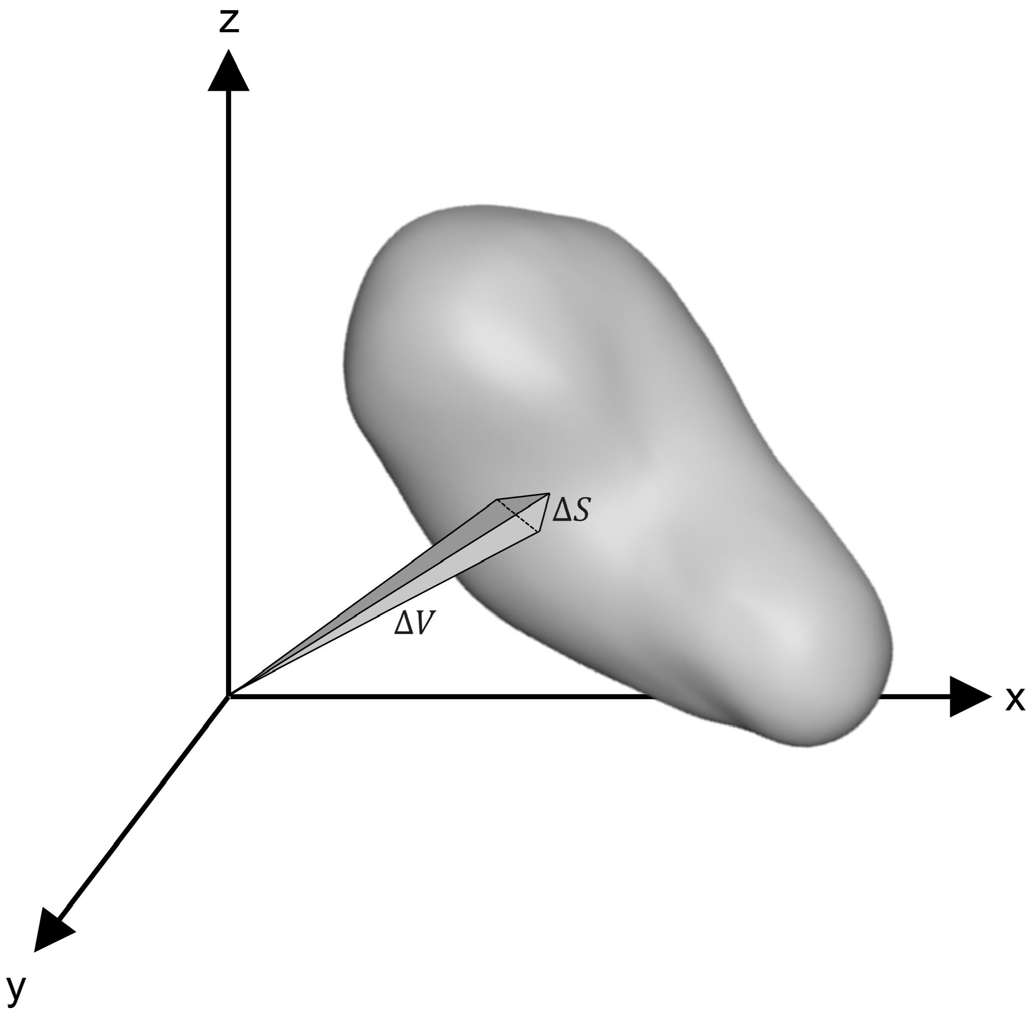
2.3.4. Power Crust Mesh Volume Computation

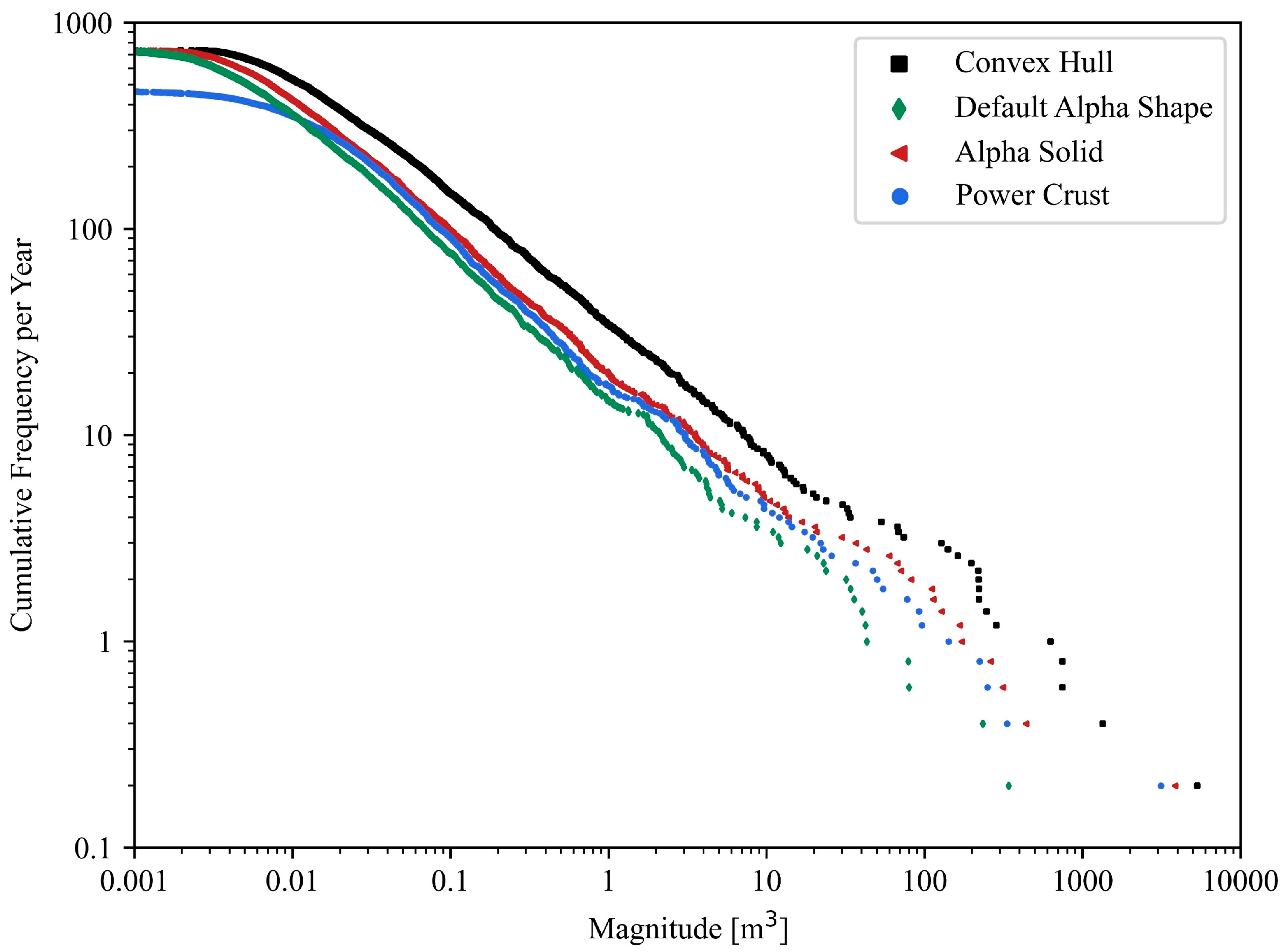
To prep the Power Crust mesh for automated volume computation, the polygonal mesh must be triangulated. To do so, we utilized the triangulation algorithm from Liepa [75] implemented within the Polygon Mesh Processing C++ library [76]. The volume of the triangulated Power Crust mesh can then be determined using the divergence theorem, in which the volume enclosed by the surface can be given by a surface integral of its vector field:

$$\underset{R}{\overset{ }{{\displaystyle \iiint }}}(\nabla ·F)dV=\underset{S}{\overset{ }{{\displaystyle \iint }}}\left(F·\widehat{n}\right)dS$$

(3)

where the $R$ is a solid region (subset of ${ℝ}^3$), $S$ is its surface boundary with local normal vectors $\widehat{n}$, and $F$ is a continuously differentiable vector field defined on a neighbourhood of $R$. The divergence theorem states that the total divergence of $F$ across the region, is equal to the flux of $F$ across its surface.

For a closed triangulated surface mesh, the divergence theorem expands one sixth of the sum of all triple products, given by each triangulated facet, presented in Equation (4) on the following page. Geometrically, this is equivalent to the sum of signed tetrahedra [77], with the apex of each mesh facet placed at the origin (illustrated in Figure 7).

Incorrect mesh facet orientations can produce sign errors, and thus inaccuracies in the volume computation. Following the right-hand rule, all mesh facet normals should point to the interior of the object, or all normals should point to the exterior of the object. It is possible for the resulting summation of tetrahedrons to be negative, therefore we take the absolute value of the volume. Holes in the mesh cause there to be some volume unaccounted for—since volumes are signed, holes can either result in an overestimation or underestimation of volume. This, however, is not an issue for the Power Crust because it is guaranteed to be 2-manifold and watertight.

$$\begin{gathered} V= {\displaystyle \sum }_i^n\frac{\left(a_i-d_i\right)·\left(\left(b_i-d_i\right) \times \left(c_i-d_i\right)\right)}{6} \\ V= \frac{1}{6}{\displaystyle \sum }_i^n{a}_i·\left(b_i\times c_i\right) \\ where d_i=\left(0,0,0\right) \end{gathered}$$

(4)

It should be noted that achieving consistent orientation for a 2-manifold watertight mesh is trivial. For all edges p1p2, there should be a compliment edge p2p1 which is part of an adjacent facet. We compute the volume utilizing the mesh data structures provided by the Polygon Mesh Processing C++ library [76].

3. Results

Rockfall volume was calculated using each of the four surface reconstruction methods, for the database of rockfalls detected during the 5-year monitoring period. The surface reconstruction results, for the largest rockfall point cloud extracted, are highlighted in Figure 8. Figure 8a shows the extracted point cloud, comprised of 98,903 points, which is shaded corresponding to its change detection signature. The Convex Hull (Figure 8b) drastically overestimated the shape across concave geometries as expected and thus overestimated the volume with an estimate of 5331 m³.

The Default Alpha Shape (Figure 8c) captured the detailed surface information of the point cloud, although, it underestimated the volume by an order of magnitude, with an estimate of 341 m³ in comparison to the estimates of 3851 m³ from the Alpha Solid and 3133 m³ from the Power Crust. The issue causing this underestimation of volume has to do with the definition of the Default Alpha Radius, and the definition of a Delaunay tetrahedron. As noted in the methods section, the Default Alpha Radius is prescribed to be sufficiently high in order to connect all point within a singular the Alpha Shape. A Delaunay tetrahedron is defined by the connection of 4-points, if they can be bounded by an empty circumsphere with a radius less than the value of Alpha (i.e., Figure 4). Restricted Voronoi Cells (i.e., Figure 4d and Figure 5) do not intersect in the interior of the Default Alpha Shape when the Default Alpha Radius is not larger than roughly ½ of the “thickness” of the rockfall point cloud—where the point cloud object “thickness” is the maximum distance which a Delaunay tetrahedron must span in order to bridge occupy the interior of the point cloud. The Default Alpha Radius is a function of the point cloud spacing, and thus has no correspondence with the thickness of the point cloud. Therefore, a point cloud with a thickness greater than roughly two-times the point spacing, will have Delaunay tetrahedra missing from its interior, where the majority of the shape’s volume is contained. The volumetric estimates of the Default Alpha Shape are therefore very poor in the instance of rockfall point clouds which have large thicknesses relative to their point spacing—even though the Default Alpha Shape seems to capture the detailed topological connections along the surface of the shape (Figure 8c). Further, the Default Alpha Shape tetrahedra are unable to bridge across large sections of missing surface information. This is revealed by the presence of holes in the Default Alpha Shape (Figure 8c). Sections of missing information in the point cloud therefore also result in underestimated Default Alpha Shape volumes.

The Alpha Solid (Figure 8d) was capable of guaranteeing that the resulting shape was 2-manifold and watertight, thus well approximating the global shape. With rockfall point clouds that have large thicknesses relative to their point spacing, the value of Alpha Radius must be fairly high in order to connect Delaunay tetrahedra across the point cloud. In the instance of these relatively thick point clouds, the Alpha Solid is therefore likely to over-interpolate across concave geometries. The surface detail of the Alpha Solid relative to the Default Alpha Shape and the Power Crust is shown in Figure 8.

The Power Crust was much more suitable for reconstructing the surface of thick point clouds with prominent concave geometric features on its surface. This is the advantage of the Power Diagram; unique weights allow for localized increases in mesh resolution where information is abundant. The Power Crust is able to create connectivity across the missing (occluded) information, while making use of the detailed surface information when it is available.

The four resulting databases were compared on a rank-frequency plot, shown in Figure 9. Differences in the surface reconstruction volume estimation are illustrated by the x-axis shift between the relations. The slope of each relation, corresponding to the power-law scaling parameter, remained relatively similar. The Convex Hull continuously overestimated the rockfall volume as expected and the Default Alpha Shape continuously underestimated the rockfall volume. On average, the Default Alpha Shape volume was 50% less than its corresponding Alpha Solid volume. The Default Alpha Shape became more noticeably erroneous with the larger point clouds. The Power Crust algorithm failed to successfully reconstruct 1237 rockfall point clouds, shown by its lower maximum cumulative frequency (Figure 9). The Power Crust failed reconstructions were for small scale point clouds with smaller volumes. A total of 95% of Power Crust failures occurred for point clouds with (1) less than 40 points or with (2) corresponding Alpha Solid volume estimates less than 2.6 × 10⁻² m³.

Power-law model scaling parameters were determined with the maximum likelihood estimation (MLE) method using a minimized Kolmogorov–Smirnov statistic for the optimal value of $x_{min}$ (see Appendix A for methodology). The truncated datasets along with their power-law models are presented in Figure 10a, where it is seen that the power-law model does not well-reflect the tail-end of the empirical distribution. Therefore, a second set of power-law models were created, aimed at improving the power-law fit to the higher magnitude data points, using a lower-bound cut-off of 1m³ (Figure 10b).

The parameters determined for each set of power-law models are presented in

Table 2. Upper: power-law PDF fits for each of the datasets utilizing the Kolmogorov–Smirnov statistic for estimating $x_{min}$ and the MLE of the scaling parameter; Lower: annual rockfall frequency calculations.

	Convex Hull	Default Alpha Shape	Alpha Solid	Power Crust	Power Crust Substituted 1
$x_{min}$ [m3]	0.0501	0.0272	0.0339	0.0279	0.0217
$b$	1.6315	1.7193	1.6808	1.7012	1.7080
	$f\left(V_1<V<V_2\right)$ [Rockfalls per Year]
$0.01 {\mathrm{m}}^3<V<0.1 {\mathrm{m}}^3$	494	327	374	366	382
$0.1 {\mathrm{m}}^3<V<1 {\mathrm{m}}^3$	115	62.4	77.9	72.8	74.8
$1 {\mathrm{m}}^3<V<10 {\mathrm{m}}^3$	26.9	11.9	16.2	14.5	14.6

¹ Failed Power Crust reconstructions substituted with the Alpha Solid volumes.

and

Table 3. Upper: Power-law PDF fits for each of the datasets utilizing MLE with a defined $x_{min}$ of 1 m³; Lower: annual rockfall frequency calculations.

	Convex Hull	Default Alpha Shape	Alpha Solid	Power Crust 1
$x_{min}$ [m3]	1	1	1	1
$b$	1.6001	1.6471	1.5743	1.5757
	$f\left(V_1<V<V_2\right)$ [Rockfalls per Year]
$1 {\mathrm{m}}^3<V<10 {\mathrm{m}}^3$	25.6	11.3	14.3	12.6
$10 {\mathrm{m}}^3<V<100 {\mathrm{m}}^3$	6.41	2.54	3.82	3.35
$100 {\mathrm{m}}^3<V<1000 {\mathrm{m}}^3$	1.61	0.573	1.02	0.890
$1000 {\mathrm{m}}^3<V<10,000 {\mathrm{m}}^3$	0.403	0.129	0.272	0.236

¹ No Power Crust failed reconstructions occurred above the 1 m³ value of $x_{min}$.

, where a higher scaling parameter indicates an increased proportion of smaller rockfall events in the distribution. A power-law model with a minimized Kolmogorov–Smirnov statistic was also fitted to the Power Crust dataset substituted with the Alpha Solid volume data, in the case of a reconstruction failure (Table 2). The Alpha Solid was used as a substitute because it is a reliable method for determining the volume of the small-scale point clouds, which challenged the Power Crust method. A smaller value of Alpha is required for the 2-manifold watertight reconstruction of small-scale point clouds. Therefore, the Alpha Solid is unlikely to interpolate across concave features in the small-scale point clouds. Additionally, the smaller scale point clouds have less potential for complex geometry. No Power Crust failures occurred above 1m³ and therefore an Alpha Solid volume substitution dataset was not created for the second set of power-law models.

The power-law models were used to determine the annual frequency of rockfall occurrence across a range of magnitudes, which is a common practice in rockfall hazard and risk analyses [6,7]. We applied the models in the domain over which they represent the datasets well, in order to better reflect the differences at the tail end of the datasets. As such, we utilized the minimized Kolmogorov–Smirnov models (Table 2) to estimate the lower magnitude ranges, and the 1m³ cut-off models (Table 3) to estimate the larger magnitude ranges. It is, however, up for discussion as to which model would be better in practice for determining the return period of the larger magnitude events, considering the history of the study site, as we note in the Discussion Section.

The variation in the annual frequencies of rockfall, shows that the surface reconstruction techniques have an impact on the assessment of rockfall hazards, and thus on risk analysis as well. The surface reconstruction techniques could also impact infrastructure design, in cases where design criteria are derived from the magnitude-frequency relation, given a return period (i.e., designing for the 50-year rockfall event).

4. Discussion

There is a significant variation in the properties of a rockfall database and its fitted power-law model, corresponding to the surface reconstruction volume estimation method utilized. We have shown that these variations have a direct impact on the estimation of the temporal frequency component of rockfall hazard determined with a magnitude-frequency analysis.

The Alpha Solid method guarantees a 2-manifold watertight reconstruction of the point clouds. However, due to the rigid usage of a maximum Voronoi cell extent by the Alpha Shape algorithm, the Delaunay Triangulation tends to over-interpolate across prominent concave geometry features in instances when the Alpha Radius must be relatively high in comparison to the point spacing. As smaller point clouds have a limited opportunity for complex concave geometry, the Alpha Solid method was very suitable for the small point clouds for which the Power Crust algorithm was unsuccessful. The potential for the Alpha Solid to have significant over-interpolations is attributed to the presence of concave features, in addition to the thickness of the point cloud object. If the thickness of the rockfall point cloud is roughly the same as the point density, then no significant over-interpolations are possible.

The Convex Hull method overestimates the rockfall volume across all scales due to significant interpolation across concave features. In the absence of concave features, and with a point cloud thickness roughly equal to the point spacing, the Convex Hull would be equivalent to the Alpha Solid.

The Default Alpha Shape method performs worse with larger rockfall point clouds that typically have more challenging geometries and higher thicknesses relative to their point spacing. With these point clouds objects, the Delaunay tetrahedra of the Default Alpha Shape are unable to bridge the thickness, thus producing internal voids that cause for an underestimation the volume (Figure 8).

We determined that the Power Crust algorithm is the best performing algorithm for the reconstruction of large-scale rockfall point clouds with significant concave geometric features. The use of a Power Diagram permits mesh connections to be detailed where there is abundant spatial information. A total of 95% of Power Crust failures occurred for point clouds with less than 40 points, and 95% of the failures occurred for point clouds with a corresponding Alpha Solid volume less than 2.6 × 10⁻² m³. As smaller scale rockfalls have surfaces closer to their medial axis, whilst the point spacing is relatively uniform (i.e., subsampled to 10 cm), our survey resulted in the smaller rockfall point clouds not having sufficient sampling for the Power Crust algorithm. This is also partially due to the reality that data resolution is not a typical constraint within the field of surface reconstruction; the Power Crust algorithm was not designed to reconstruct extremely small point clouds with relatively low data resolution. Keep in mind that the typical point spacing for the TLS surveys was subsampled to 10 cm and the limit of detection was 5 cm. Different point clouds causing failed Power Crust reconstructions are to be expected with different data resolutions and limits of detection.

It is possible to provide quantitative evaluations of the surface reconstruction accuracy, for individual point clouds. This was demonstrated in the previous study conducted by Bonneau et al. [50]. To do so, the volume must be known, and therefore digital surface representation of the object must be known. The degree to which conclusions can be made, however, is case specific and sensitive, considering the synthetic object tested. The degree of error found in the methods is closely tied to the geometry of the synthetic object, the point cloud sampling density, and the presence of point cloud imperfections, as we discuss in this article. For this reason, the authors believe that the application of surface reconstruction across a wide spectrum of real rockfall point clouds allows for a better representation of the potential errors in volume estimation, in comparison to the detailed quantitative analysis possible with hand-picked synthetic objects.

In the previous study conducted by Bonneau et al. [50], the importance of surface reconstruction for volume estimation was demonstrated using three real rockfall objects ranging from approximately 1 to 120 m³. In this work, we found similar results, however, the larger scale of analysis (i.e., 3668 rockfalls ranging from approx. 0.001 to 3000 m³) allow us to make much broader conclusions concerning the development of magnitude–frequency relations. We observed significant overestimates in the Alpha Solid volume, due to larger-scale point clouds with significant concave features. For the largest rockfall tested, Bonneau et al. [50] saw a 5% larger estimate in volume by of the Alpha Solid in comparison to the Power Crust. The largest event presented in the current study had an Alpha Solid reconstruction with a 23% larger estimate (Figure 8). This study therefore demonstrates that the Power Crust is the better method to use on large-scale point clouds.

While Bonneau et al. did not experience any issues utilizing the Power Crust algorithm and considered it to be the best method, we determined that small-scale point clouds can result in failed reconstructions, requiring for a hybrid methodology which utilizes the Alpha Solid reconstruction on small-scale point clouds. The potential for complex topological connections in small point clouds is small. Therefore, it makes sense that the simpler Alpha Solid method should be suitable for reconstructing the smaller point clouds. It is imperative that bounding box checks are completed on the outputted Power Crust meshes, to ensure that the algorithm did not mislabel the poles, as it can drastically alter the volume estimate.

Surface reconstruction for volumetric estimates will remain a challenge in natural environments due to all the factors that can contribute to erroneous reconstruction. There are many algorithms that have been presented in the computational geometry and computer vision fields [48] that have yet to be tested for automated volumetric estimation for rockfall events. To date, rockfall related work in this area has focused on the use of explicit polyhedron representations determined using computational geometry. Menegoni et al. [79] present the use of Poisson’s reconstruction [80] to back analyze a rockfall event that occurred in the Western Italian Alps. This case demonstrates that implicit surface representations can also be used for rockfall volumetric estimation. Although, for Poisson’s reconstruction, point-normal estimates with correct orientation must be provided as input, and a voxel size used for the Marching Cubes algorithm [53] variant must be specified. This adds a further level of complexity to an automated 3D rockfall volume calculation system, as the determination of optimal scales for the geometric point cloud operators remains a consistent challenge. Further work is required to investigate the viability of implicit and explicit surface reconstruction by comparing their precision, accuracy, and ability to automate. Nevertheless, a sound understanding of the processes and algorithms being used to facilitate the surface reconstruction and subsequent volume estimates is needed in order to have confidence in digital rockfall databases and their resulting magnitude-frequency relations.

All things considered, given a rockfall database with volume estimates, there remains the crucial step in building a magnitude-frequency model. We utilized the maximum likelihood estimation technique (Appendix A), which is robust in determining the scaling and resulting normalization parameter [11,81]. Determining an appropriate lower bound truncation on the dataset is important, as there is a rollover point in the magnitude-frequency behaviour of rockfall inventories. The Kolmogorov–Smirnov test (Appendix A) determined an optimal minimum truncation. In practice, goodness of fit tests are necessary to determine whether an empirical dataset is in fact best modeled using a power-law distribution [11]. Validation for this study was simply completed in a qualitative manner considering the wide acceptance of power-law models for rockfall in the literature, and given our goal to compare volume estimation methods.

For this dataset it was noted that the empirical data do not agree with the power-law towards the tail-end of the distribution, and we have considered whether this is due to natural behavior, statistical bias, or error in the methods. Firstly, this rock slope has had a recent history of significant large-scale failures, including a 50,000 m³ rockslide in November of 2012 [60], and an approximate 3000 m³ rockfall in December of 2014 (i.e., Figure 8). The large failures would have destabilized a significant section of the rock mass. The increased proportion of large rockfall events may have been further amplified by the fact that this rock slope was monitored throughout a highly active time period (November 2013 – December 2018). The 50,000m³ rockslide was not included in the magnitude-frequency relations because it is a different classification of landslide with fundamentally different mechanisms [2].

In regard to errors in the methods, longer intervals between data collection for this site may permit several proximal smaller volume rockfalls to be clustered together as a singular event [18,39], thus increasing the proportion of large rockfall events in the distribution. Lastly, natural geological factors could also be at play for increasing the proportion of large magnitude events, considering the elevated activity of the site. The moderate spacing of wedge forming joints, and presence of local faults [60] could form blocks which fail at relatively higher frequencies than those forecasted by the power-law. The further investigation of these hypotheses requires the continued monitoring of the site as it adapts following the recent activities in rockfall. Increasing monitoring frequency will give a truer reflection of the rockfall activity without the artifacts of coalescing rockfalls. Further understanding the geostructural and geomechanical characteristics contributing to rock mass failure will also aid in further understanding the magnitude-frequency distribution of rockfall at the site.

5. Conclusions

With the development of cheaper remote sensing platforms capable of capturing detailed spatial information of near vertical rock cliffs, comes the opportunity to rigorously monitor and understand rock slope hazards across larger areas of mountainous terrain. The coevolution of modern computing hardware and 3D software has provided the capability to rapidly, and intuitively, process the data acquisition. Over the past decade, more custom tools have been created to extract important information from the processed datasets, in order to further our understanding of rock slope hazards. One of these tools has been the extraction of rockfall from these datasets in 3D, in which the occurrences can be assembled into a rockfall database providing critical information pertaining to rockfall hazard. This work was started by Tonini and Abellán [45], and has since been improved by many complementary studies [18,34,36,38,40,50]. In further developing these tools, there is a need to reduce the amount of error present in the systems which document rockfall occurrence, as they can have a direct implication on our measure of rockfall hazard. Thus, errors can further impact risk mitigation decisions, and infrastructure design criteria. With evolving methods, there has been a push to increase the portion of tools to be fully 3D, rather than rasterized (2.5D). We showed that the determination of volume for rockfall point clouds is a difficult task, considering the presence of point cloud imperfections generated as a result of the instruments, survey design, processing, and rockfall extraction algorithms. We summarized four different computational geometry surface reconstruction techniques, used to create a digital representation of the rockfalls and determine their respective volumes.

We determined that the Alpha Solid technique is simple enough to provide an accurate estimation of rockfall volumes of small-scale point clouds beneath 40 points, with our 10 cm point spacing and 5 cm limit of detection. The Alpha Solid method will begin to overestimate the volume of larger point clouds with prominent convex geometry features due to over-interpolation. We determined that the Power Crust algorithm is a much better approach for large-scale point clouds with prominent convex geometry. The Power Crust algorithm is more likely to fail the reconstruction on small-scale point clouds, which do not have sufficiently dense sampling relative to their curvature (i.e., a small distance from the surface to their medial axis). As such, we provided a robust workflow to ensure that the incorrect reconstructions are rejected from the database. The optimal surface reconstruction method for computing rockfall volume in 3D was determined to be the Power Crust method, substituted with the Alpha Solid method for the small-scale point clouds with insufficient sampling density and non-complex geometry.

References

1. Varnes, D.J. Slope Movement Types and Processes. Transp. Res. Board Natl. Acad. Sci. Spec. Rep. 1978, 176, 11–33. [Google Scholar]
2. Hungr, O.; Leroueil, S.; Picarelli, L. The Varnes Classification of Landslide Types, an Update. Landslides 2014, 11, 167–194. [Google Scholar] [CrossRef]
3. Volkwein, A.; Schellenberg, K.; Labiouse, V.; Agliardi, F.; Berger, F.; Bourrier, F.; Dorren, L.; Gerber, W. Rockfall Characterisation and Structural Protection—A Review. Nat. Hazards Earth Syst. Sci. 2011, 2617–2651. [Google Scholar] [CrossRef] [Green Version]
4. Corominas, J.; Moya, J. A Review of Assessing Landslide Frequency for Hazard Zoning Purposes. Eng. Geol. 2008, 102, 193–213. [Google Scholar] [CrossRef]
5. Corominas, J.; Copons, R.; Moya, J.; Vilaplana, J.M.; Altimir, J.; Amigó, J. Quantitative Assessment of the Residual Risk in a Rockfall Protected Area. Landslides 2005, 2, 343–357. [Google Scholar] [CrossRef]
6. Guzzetti, F.; Reichenbach, P.; Ghigi, S. Rockfall Hazard and Risk Assessment Along a Transportation Corridor in the Nera Valley, Central Italy. Environ. Manag. 2004, 34, 191–208. [Google Scholar] [CrossRef] [PubMed]
7. Hungr, O.; Evans, S.G.; Hazzard, J. Magnitude and Frequency of Rock Falls and Rock Slides along the Main Transportation Corridors of Southwestern British Columbia. Can. Geotech. J. 1999, 36, 224–238. [Google Scholar] [CrossRef]
8. Corominas, J.; Mavrouli, O.; Ruiz-Carulla, R. Magnitude and Frequency Relations: Are There Geological Constraints to the Rockfall Size? Landslides 2018, 15, 829–845. [Google Scholar] [CrossRef] [Green Version]
9. Malamud, B.D.; Turcotte, D.L.; Guzzetti, F.; Reichenbach, P. Landslide Inventories and Their Statistical Properties. Earth Surf. Process. Landf. 2004, 711, 687–711. [Google Scholar] [CrossRef]
10. Guthrie, R.H.; Evans, S.G. Analysis of Landslide Frequencies and Characteristics in a Natural System, Coastal British Columbia. Earth Surf. Process. Landf. 2004, 29, 1321–1339. [Google Scholar] [CrossRef]
11. Clauset, A.; Shalizi, C.R.; Newman, M.E.J. Power-Law Distributions in Empirical Data. SIAM Rev. 2009, 51, 661–703. [Google Scholar] [CrossRef] [Green Version]
12. Brardinoni, F.; Church, M. Representing the Landslide Magnitude–Frequency Relation: Capilano River Basin, British Columbia. Earth Surf. Process. Landf. 2004, 29, 115–124. [Google Scholar] [CrossRef]
13. Hovius, N.; Stark, C.P.; Hao-Tsu, C.; Jiun-Chuan, L. Supply and Removal of Sediment in a Landslide-Dominated Mountain Belt: Central Range, Taiwan. J. Geol. 2000, 108, 73–89. [Google Scholar] [CrossRef] [PubMed]
14. Martin, Y.; Rood, K.; Schwab, J.W.; Church, M. Sediment Transfer by Shallow Landsliding in the Queen Charlotte Islands, British Columbia. Can. J. Earth Sci. 2002, 39, 189–205. [Google Scholar] [CrossRef] [Green Version]
15. Pelletier, J.D.; Malamud, B.D.; Blodgett, T.; Turcotte, D.L. Scale-Invariance of Soil Moisture Variability and Its Implications for the Frequency-Size Distribution of Landslides. Eng. Geol. 1997, 48, 255–268. [Google Scholar] [CrossRef]
16. Guthrie, R.H.; Evans, S.G. Magnitude and Frequency of Landslides Triggered by a Storm Event, Loughborough Inlet, British Columbia. Nat. Hazards Earth Syst. Sci. 2004, 4, 475–483. [Google Scholar] [CrossRef]
17. Stark, C.P.; Hovius, N. The Characterization of Landslide Size Distributions. Geophys. Res. Lett. 2001, 28, 1091–1094. [Google Scholar] [CrossRef]
18. Williams, J.G.; Rosser, N.J.; Hardy, R.J.; Brain, M.J. The Importance of Monitoring Interval for Rockfall Magnitude-Frequency Estimation. J. Geophys. Res. Earth Surf. 2019, 124, 2841–2853. [Google Scholar] [CrossRef] [Green Version]
19. Stoffel, M.; Schneuwly, D.; Bollschweiler, M.; Lièvre, I.; Delaloye, R.; Myint, M.; Monbaron, M. Analyzing Rockfall Activity (1600–2002) in a Protection Forest—A Case Study Using Dendrogeomorphology. Geomorphology 2005, 68, 224–241. [Google Scholar] [CrossRef]
20. Rosser, N.J.; Lim, M.; Petley, D.; Dunning, S.; Allison, R. Patterns of Precursory Rockfall Prior to Slope Failure. J. Geophys. Res. 2007, 112, F04014. [Google Scholar] [CrossRef]
21. Nichol, J.; Wong, M.S. Satellite Remote Sensing for Detailed Landslide Inventories Using Change Detection and Image Fusion. Int. J. Remote Sens. 2005, 26, 1913–1926. [Google Scholar] [CrossRef]
22. Lu, P.; Stumpf, A.; Kerle, N.; Casagli, N. Object-Oriented Change Detection for Landslide Rapid Mapping. IEEE Geosci. Remote Sens. Lett. 2011, 8, 701–705. [Google Scholar] [CrossRef]
23. Kromer, R.A.; Hutchinson, D.J.; Lato, M.J.; Gauthier, D.; Edwards, T. Identifying Rock Slope Failure Precursors Using LiDAR for Transportation Corridor Hazard Management. Eng. Geol. 2015, 195, 93–103. [Google Scholar] [CrossRef]
24. Warrick, J.A.; Ritchie, A.C.; Adelman, G.; Adelman, K.; Limber, P.W. New Techniques to Measure Cliff Change from Historical Oblique Aerial Photographs and Structure-from-Motion Photogrammetry. J. Coast. Res. 2017, 33, 39. [Google Scholar] [CrossRef] [Green Version]
25. Lato, M.J.; Hutchinson, D.J.; Gauthier, D.; Edwards, T.; Ondercin, M. Comparison of Airborne Laser Scanning, Terrestrial Laser Scanning, and Terrestrial Photogrammetry for Mapping Differential Slope Change in Mountainous Terrain. Can. Geotech. J. 2015, 52, 129–140. [Google Scholar] [CrossRef]
26. Benjamin, J.; Rosser, N.J.; Brain, M.J. Emergent Characteristics of Rockfall Inventories Captured at a Regional Scale. Earth Surf. Process. Landf. 2020, 45, 2773–2787. [Google Scholar] [CrossRef]
27. Kromer, R.A.; Abellán, A.; Hutchinson, D.J.; Lato, M.J.; Chanut, M.A.; Dubois, L.; Jaboyedoff, M. Automated Terrestrial Laser Scanning with Near-Real-Time Change Detection—Monitoring of the Séchilienne Landslide. Earth Surf. Dyn. 2017, 5, 293–310. [Google Scholar] [CrossRef] [Green Version]
28. Kromer, R.A.; Walton, G.; Gray, B.; Lato, M.J.; Group, R. Development and Optimization of an Automated Fixed-Location Time Lapse Photogrammetric Rock Slope Monitoring System. Remote Sens. 2019, 11, 1890. [Google Scholar] [CrossRef] [Green Version]
29. Eltner, A.; Kaiser, A.; Abellan, A.; Schindewolf, M. Time Lapse Structure-from-Motion Photogrammetry for Continuous Geomorphic Monitoring. Earth Surf. Process. Landf. 2017, 42, 2240–2253. [Google Scholar] [CrossRef]
30. Telling, J.; Lyda, A.; Hartzell, P.; Glennie, C.L. Review of Earth Science Research Using Terrestrial Laser Scanning. Earth Sci. Rev. 2017, 169, 35–68. [Google Scholar] [CrossRef] [Green Version]
31. Abellán, A.; Oppikofer, T.; Jaboyedoff, M.; Rosser, N.J.; Lim, M.; Lato, M.J. Terrestrial Laser Scanning of Rock Slope Instabilities. Earth Surf. Process. Landf. 2014, 39, 80–97. [Google Scholar] [CrossRef]
32. Smith, M.W.; Carrivick, J.L.; Quincey, D.J. Structure from Motion Photogrammetry in Physical Geography. Prog. Phys. Geogr. Earth Environ. 2016, 40, 247–275. [Google Scholar] [CrossRef] [Green Version]
33. Anderson, K.; Westoby, M.J.; James, M.R. Low-Budget Topographic Surveying Comes of Age: Structure from Motion Photogrammetry in Geography and the Geosciences. Prog. Phys. Geogr. Earth Environ. 2019, 43, 163–173. [Google Scholar] [CrossRef]
34. Guerin, A.; Ravanel, L.; Matasci, B.; Jaboyedoff, M.; Deline, P. The Three-Stage Rock Failure Dynamics of the Drus (Mont Blanc Massif, France) since the June 2005 Large Event. Sci. Rep. 2020, 10. [Google Scholar] [CrossRef]
35. Hartmeyer, I.; Keuschnig, M.; Delleske, R.; Krautblatter, M.; Lang, A.; Schrott, L.; Prasicek, G.; Otto, J.-C. A 6-Year Lidar Survey Reveals Enhanced Rockwall Retreat and Modified Rockfall Magnitudes/Frequencies in Deglaciating Cirques. Earth Surf. Dyn. 2020, 8, 753–768. [Google Scholar] [CrossRef]
36. DiFrancesco, P.-M.; Bonneau, D.A.; Hutchinson, D.J. The Implications of M3C2 Projection Diameter on 3D Semi-Automated Rockfall Extraction from Sequential Terrestrial Laser Scanning Point Clouds. Remote Sens. 2020, 12, 1885. [Google Scholar] [CrossRef]
37. Guerin, A.; Stock, G.M.; Radue, M.J.; Jaboyedoff, M.; Collins, B.D.; Matasci, B.; Avdievitch, N.; Derron, M.-H. Quantifying 40 Years of Rockfall Activity in Yosemite Valley with Historical Structure-from-Motion Photogrammetry and Terrestrial Laser Scanning. Geomorphology 2020, 356, 107069. [Google Scholar] [CrossRef]
38. Williams, J.G.; Rosser, N.J.; Hardy, R.J.; Brain, M.J.; Afana, A.A. Optimising 4-D Surface Change Detection: An Approach for Capturing Rockfall Magnitude-Frequency. Earth Surf. Dyn. 2018, 6, 101–119. [Google Scholar] [CrossRef] [Green Version]
39. van Veen, M.; Hutchinson, D.J.; Kromer, R.; Lato, M.; Edwards, T. Effects of Sampling Interval on the Frequency—Magnitude Relationship of Rockfalls Detected from Terrestrial Laser Scanning Using Semi-Automated Methods. Landslides 2017, 14, 1579–1592. [Google Scholar] [CrossRef]
40. Olsen, M.J.; Wartman, J.; McAlister, M.; Mahmoudabadi, H.; O’Banion, M.; Dunham, L.; Cunningham, K. To Fill or Not to Fill: Sensitivity Analysis of the Influence of Resolution and Hole Filling on Point Cloud Surface Modeling and Individual Rockfall Event Detection. Remote Sens. 2015, 7, 12103–12134. [Google Scholar] [CrossRef] [Green Version]
41. Carrea, D.; Abellan, A.; Derron, M.-H.; Jaboyedoff, M. Automatic Rockfalls Volume Estimation Based on Terrestrial Laser Scanning Data. In Engineering Geology for Society and Territory—Volume 2; Springer International Publishing: Cham, Switzerland, 2015; pp. 425–428. [Google Scholar] [CrossRef]
42. Cignoni, P.; Rocchini, C.; Scopigno, R. Metro: Measuring Error on Simplified Surfaces. Comput. Graph. Forum 1998, 17, 167–174. [Google Scholar] [CrossRef] [Green Version]
43. Lague, D.; Brodu, N.; Leroux, J. Accurate 3D Comparison of Complex Topography with Terrestrial Laser Scanner: Application to the Rangitikei Canyon (N-Z). ISPRS J. Photogramm. Remote Sens. 2013, 82, 10–26. [Google Scholar] [CrossRef] [Green Version]
44. Ester, M.; Kriegel, H.P.; Sander, J.; Xu, X. A Density-Based Algorithm for Discovering Clusters in Large Spatial Databases with Noise. In Proceedings of the Second International Conference on Knowledge Discovery and Data Mining, Portland, OR, USA, 2–4 August 1996; Simoudis, E., Fayyad, U., Han, J., Eds.; AAAI Press: Menlo Park, CA, USA, 1996; pp. 226–231. [Google Scholar]
45. Tonini, M.; Abellán, A. Rockfall Detection from Terrestrial LiDAR Point Clouds: A Clustering Approach Using R. J. Spat. Inf. Sci. 2014, 8. [Google Scholar] [CrossRef]
46. Hoppe, H.; DeRose, T.; Duchamp, T.; McDonald, J.; Stuetzle, W. Surface Reconstruction from Unorganized Points. Comput. Graph. 1992, 26, 71–78. [Google Scholar] [CrossRef]
47. Benjamin, J.; Rosser, N.J.; Brain, M. Rockfall Detection and Volumetric Characterisation Using LiDAR. In Landslides and Engineered Slopes. Experience, Theory and Practice; CRC Press: Naples, Italy, 2016; pp. 389–395. [Google Scholar] [CrossRef]
48. Berger, M.; Tagliasacchi, A.; Seversky, L.M.; Alliez, P.; Levine, J.A.; Sharf, A.; Silva, C.T. State of the Art in Surface Reconstruction from Point Clouds. In Eurographics 2014—State of the Art Reports; Lefebvre, S., Spagnuolo, M., Eds.; The Eurographics Association: Strasbourg, France, 2014; pp. 161–185. [Google Scholar] [CrossRef]
49. Edelsbrunner, H.; Harer, J. Computational Toplogy an Introduction; American Mathematical Society: Providence, RI, USA, 2010. [Google Scholar]
50. Bonneau, D.A.; DiFrancesco, P.-M.; Hutchinson, D.J. Surface Reconstruction for Three-Dimensional Rockfall Volumetric Analysis. ISPRS Int. J. Geo Inf. 2019, 8, 548. [Google Scholar] [CrossRef] [Green Version]
51. Zhao, H.-K.; Osher, S.; Fedkiw, R. Fast Surface Reconstruction Using the Level Set Method. In Proceedings of the IEEE Workshop on Variational and Level Set Methods in Computer Vision, Vancouver, BC, Canada, 13 July 2001; IEEE Computer Society: Washington, DC, USA, 2001; pp. 194–201. [Google Scholar] [CrossRef] [Green Version]
52. Kazhdan, M. Reconstruction of Solid Models from Oriented Point Sets. In Proceedings of the Third Eurographics Symposium on Geometry Processing, SGP ’05, Vienna, Austria, 4–6 July 2005; pp. 73–82. [Google Scholar]
53. Lorensen, W.E.; Cline, H.E. Marching Cubes: A High Resolution 3D Surface Construction Algorithm. In Proceedings of the 14th Annual Conference on Computer Graphics and Interactive Techniques—SIGGRAPH ’87, Anaheim, CA, USA, 27–31 July 1987; ACM Press: New York, NY, USA, 1987; pp. 163–169. [Google Scholar] [CrossRef]
54. Amenta, N.; Bern, M.; Kamvysselis, M. A New Voronoi-Based Surface Reconstruction Algorithm. In Proceedings of the 25th Annual Conference on Computer Graphics and Interactive Techniques—SIGGRAPH ’98, Orlando, FL, USA, 19–24 July 1998; ACM Press: New York, NY, USA, 1998; pp. 415–421. [Google Scholar] [CrossRef] [Green Version]
55. Amenta, N.; Choi, S.; Kolluri, R.K. The Power Crust. In Proceedings of the Sixth ACM Symposium on Solid Modeling and Applications—SMA ’01, Ann Arbor, MI, USA, 4–8 June 2001; ACM Press: New York, NY, USA, 2001; pp. 249–266. [Google Scholar] [CrossRef]
56. Edelsbrunner, H.; Mücke, E.P. Three-Dimensional Alpha Shapes. ACM Trans. Graph. 1994, 13, 43–72. [Google Scholar] [CrossRef]
57. Boissonnat, J.-D. Geometric Structures for Three-Dimensional Shape Representation. ACM Trans. Graph. 1984, 3, 266–286. [Google Scholar] [CrossRef]
58. MacLaurin, C.I.; Mahoney, J.B.; Haggart, J.W.; Goodin, J.R.; Mustard, P.S. The Jackass Mountain Group of South-Central British Columbia: Depositional Setting and Evolution of an Early Cretaceous Deltaic Complex. Can. J. Earth Sci. 2011, 48, 930–951. [Google Scholar] [CrossRef]
59. Kromer, R.A.; Lato, M.J.; Hutchinson, D.J.; Gauthier, D.; Edwards, T. Managing Rockfall Risk through Baseline Monitoring of Precursors with a Terrestrial Laser Scanner. Can. Geotech. J. 2017, 967. [Google Scholar] [CrossRef]
60. Sturzenegger, M.; Keegan, T.; Wen, A.; Willms, D.; Stead, D.; Edwards, T. LiDAR and Discrete Fracture Network Modeling for Rockslide Characterization and Analysis. In Engineering Geology for Society and Territory—Volume 6; Springer International Publishing: Cham, Switzerland, 2015; pp. 223–227. [Google Scholar] [CrossRef]
61. Teledyne Optech. ILRIS Summary Specification Sheet; Teledyne Optech: Vaughan, ON, Canada, 2014. [Google Scholar]
62. Pesci, A.; Teza, G.; Bonali, E. Terrestrial Laser Scanner Resolution: Numerical Simulations and Experiments on Spatial Sampling Optimization. Remote Sens. 2011, 3, 167–184. [Google Scholar] [CrossRef] [Green Version]
63. Riegl Laser Measurement Systems. Riegl VZ-400i Datasheet; Riegl Laser Measurement Systems: Horn, Austria, 2017. [Google Scholar]
64. Devert, A. 2D Laguerre-Voronoi Diagrams. Available online: https://gist.github.com/marmakoide/45d5389252683ae09c2df49d0548a627 (accessed on 10 January 2021).
65. Royer, A. Mesh Generation with Alpha Complexes. Available online: http://ameroyer.github.io/projects/2018/03/01/alphacomplexes.html (accessed on 11 January 2021).
66. Virtanen, P.; Gommers, R.; Oliphant, T.E.; Haberland, M.; Reddy, T.; Cournapeau, D.; Burovski, E.; Peterson, P.; Weckesser, W.; Bright, J.; et al. SciPy 1.0: Fundamental Algorithms for Scientific Computing in Python. Nat. Methods 2020, 17, 261–272. [Google Scholar] [CrossRef] [Green Version]
67. Hunter, J.D. Matplotlib: A 2D Graphics Environment. Comput. Sci. Eng. 2007, 9, 90–95. [Google Scholar] [CrossRef]
68. Edelsbrunner, H. Voronoi Diagrams. In Algorithms in Combinatorial Geometry; Springer: Berlin/Heidelberg, Germany, 1987; pp. 293–335. [Google Scholar] [CrossRef]
69. Mathworks. MATLAB—Version 9.9 (r2020b). 2020. Available online: https://www.mathworks.com/ (accessed on 15 November 2020).
70. Bernardini, F.; Bajaj, C.L.; Chen, J.; Schikore, D.R. A Triangulation-Based Object Reconstruction Method. In Proceedings of the Thirteenth Annual Symposium on Computational Geometry—SCG ’97, Nice, France, 4–6 June 1996; ACM Press: New York, NY, USA, 1997; pp. 481–484. [Google Scholar] [CrossRef] [Green Version]
71. Amenta, N.; Choi, S.; Kolluri, R.K. The Power Crust, Unions of Balls, and the Medial Axis Transform. Comput. Geom. 2001, 19, 127–153. [Google Scholar] [CrossRef] [Green Version]
72. Alhashim, I. Power Crust—A Port for Windows. 2012. Available online: https://github.com/ialhashim/powercrust (accessed on 15 November 2020).
73. Clarkson, K. A Program for Convex Hulls. 1995. Available online: http://www.netlib.org/voronoi/hull.html (accessed on 10 December 2020).
74. Clarkson, K.L.; Shor, P.W. Applications of Random Sampling in Computational Geometry, II. Discret. Comput. Geom. 1989, 4, 387–421. [Google Scholar] [CrossRef] [Green Version]
75. Liepa, P. Filling Holes in Meshes. In Eurographics Symposium on Geometry Processing; Kobbelt, L., Schroeder, P., Hoppe, H., Eds.; The Eurographics Association: Genoa, Italy, 2003. [Google Scholar] [CrossRef]
76. Sieger, D.; Botsch, M. The Polygon Mesh Processing Library—Version 1.2.1. 2020. Available online: https://www.pmp-library.org/ (accessed on 23 December 2020).
77. Lien, S.; Kajiya, J.T. A Symbolic Method for Calculating the Integral Properties of Arbitrary Nonconvex Polyhedra. IEEE Comput. Graph. Appl. 1984, 4, 35–42. [Google Scholar] [CrossRef]
78. Blender Foundation and Community. Blender—A 3D Modelling and Rendering Package—Version 2.90.0; Stichting Blender Foundation: Amsterdam, The Netherlands, 2020; Available online: https://www.blender.org/ (accessed on 22 September 2020).
79. Menegoni, N.; Giordan, D.; Perotti, C. Reliability and Uncertainties of the Analysis of an Unstable Rock Slope Performed on RPAS Digital Outcrop Models: The Case of the Gallivaggio Landslide (Western Alps, Italy). Remote Sens. 2020, 12, 1635. [Google Scholar] [CrossRef]
80. Kazhdan, M.; Hoppe, H. Screened Poisson Surface Reconstruction. ACM Trans. Graph. 2013, 32, 1–13. [Google Scholar] [CrossRef] [Green Version]
81. Goldstein, M.L.; Morris, S.A.; Yen, G.G. Problems with Fitting to the Power-Law Distribution. Eur. Phys. J. B 2004, 41, 255–258. [Google Scholar] [CrossRef] [Green Version]
82. Benjamin, J. Regional-Scale Controls on Rockfall Occurrence. Ph.D. Thesis, Durham University, Durham, UK, 2018. Available online: http://etheses.dur.ac.uk/12813/ (accessed on 17 June 2020).
Figure 1. Point cloud imperfections known to challenge surface reconstruction algorithms: (a) The original surface being sampled; (b) Non-uniform sampling; (c) Noise; (d) Outliers; (e) Misaligned data; (f) Missing data. Adapted from Berger et al. [48].
Ijgi 10 00157 g001
Figure 2. Visual definitions of 2-manifold surfaces and planar patches, modified after Bonneau et al. [50]; (a) A continuous 2-manifold sphere with an outlined neighbourhood which is homeomorphic to a Euclidean disk; (b) A similar 2-manifold surface mesh; (c) A non-manifold mesh edge; (d) A proper manifold mesh edge; (e) A non-manifold mesh self intersection; (f) A non-manifold node connecting two tetrahedra.
Ijgi 10 00157 g002
Figure 3. Rockfall data of the CN Ashcroft Mile 109.4 study site, across a 5-year span from November 2013 to December 2018. Presented in 3 different intervals to reduce overprinting data in the visualization. An 80 m long rock shed constructed in fall of 2014 supports a talus cone which has built up, allowing rockfall fragments to pass overtop of the track. Clustered rockfall point clouds are randomly colourized and projected onto a helicopter photogrammetry point cloud (December 2014); (a) 347 days, from 28 November 2013 to 10 November 2014; (b) 104 days, from 10 November 2014 to 17 February 2015, occurrence of an approximate 3000 m3 rockfall and several other events in the hundreds of cubic meters; (c) 1381 days, from 17 February 2015 to 4 December 2018.
Ijgi 10 00157 g003
Figure 4. Key computational geometry tools presented in 2D. (a) The Voronoi diagram of the point set. Voronoi cells contain all space nearest to its sample; (b) a Power diagram, with weights denoted by the radius of the blue circle surrounding each point. Power cells contain all space, in which the distance subtracted by its cell weight (i.e., the Power distance), is less than competing cells. The cell edges of competing samples are drawn at the distance where the outer circle boundaries intersect. If all weights are equal it would result in the same diagram as in (a); (c) The Delaunay triangulation (blue), which is the dual graph of the Voronoi diagram (black). An example of an empty circumcircle (red), centered at a Voronoi vertex (red), showing that its triangulation is Delaunay; (d) A restricted Voronoi diagram (black), with a uniform weight determining the maximum extent of the cells. The resulting Delaunay triangulation (blue) is made for the trios of adjoining cells. A lack of cell adjacencies results in several points becoming excluded from the triangulation. Visualization adapted from Devert [64] and Royer [65] with the Scipy Spatial [66] and Matplotlib [67] libraries for Python.
Ijgi 10 00157 g004
Figure 5. Restricted Voronoi diagrams and their resulting Delaunay Triangulations producing the triangulated Alpha Shape, adapted from Royer [65]. (a) a zero Alpha Radius producing an empty Alpha Shape; (bh) an increase in Alpha Radius from left to right, and top to bottom, respectively; (i) an infinite Alpha Radius producing the Convex Hull. Visualization aided by the Scipy Spatial [66] and Matplotlib [67] libraries for Python.
Ijgi 10 00157 g005
Figure 6. A 2D illustration of the Power Crust algorithm, adapted from Amenta et al. [55]; (a) the object with its medial axis; (b) the sampled point cloud, S , with an inset image showing the 5-times bounding box points added to the samples; (c) the Voronoi diagram of S , with Voronoi vertices, V , plotted in blue; (d) maximal balls centered at the Voronoi vertices. The straight lines are a result of far outer polar balls with large radii such that they simplify to half-spaces intersecting the convex hull of S , (e) Power diagram of V , constructed with the weights of the maximal balls in (d). Polar balls within the envelope of another do not have their own Power cell, as they are overpowered; (f) the labelled Power diagram with the medial axis approximation. The boundary between the interior and exterior Power diagram cells is the Power Crust. Visualization adapted from Devert [64] and aided by the Scipy Spatial [66] and Matplotlib [67] libraries for Python.
Ijgi 10 00157 g006
Figure 7. A mesh facet expanded into a signed tetrahedron with its apex at the origin. Adapted from Lien and Kajiya [77].
Ijgi 10 00157 g007
Figure 8. Surface reconstruction results for the largest rockfall point cloud, with a side view (top) and a front view (bottom), rendered in Blender [78]. (a) The rockfall point cloud visualized by its change detection signature. Missing surface information in the point cloud is observed where the back (cold-coloured) points are visible through the gaps in the front (warm-coloured). Missing information occurs between the boundaries of the back and front data, and across surfaces with high incidence angles relative to the scanner; (b) The Convex Hull reconstruction; (c) The Default Alpha Shape reconstruction; (d) The Alpha Solid reconstruction; (e) The Power Crust reconstruction.
Ijgi 10 00157 g008
Figure 9. The rank-frequency (cumulative) distributions generated by each of the surface reconstruction methods, with cumulative frequencies normalized by the 5-year monitoring period. The Power Crust dataset does not include the rockfalls for which the reconstruction failed, hence its more significant rollover and unique cumulative frequency. The majority of failed reconstructions were for small-scale point clouds and thus for small volumes.
Ijgi 10 00157 g009
Figure 10. (a) the maximum likelihood estimation of power-law models, with the datasets truncated at their estimated values of x m i n found by minimizing the Kolmogorov–Smirnov statistic; (b) the maximum likelihood estimation of the power-law models, truncated at 1m3 in order to better fit the tail-end of the distribution.
Ijgi 10 00157 g010