
Mapping Grasslands in Mixed Grassland Ecoregion of Saskatchewan Using Big Remote Sensing Data and Machine Learning


1
Department of Soil Science, University of Manitoba, 13 Freedman Crescent, Winnipeg, MB R3T 2N2, Canada
2
Habitat Unit, Saskatchewan Ministry of Environment, Fish, Wildlife and Lands Branch, 3211 Albert St., Regina, SK S4S 5W6, Canada
3
Royal Saskatchewan Museum, 2340 Albert St., Regina, SK S4P 2V7, Canada
*
Author to whom correspondence should be addressed.
Remote Sens. 2021, 13(24), 4972; https://doi.org/10.3390/rs13244972
Submission received: 1 November 2021
/
Revised: 2 December 2021
/
Accepted: 5 December 2021
/
Published: 7 December 2021
(This article belongs to the Section Environmental Remote Sensing)
Abstract
:Accurate spatial distribution information of native, mixed, and tame grasslands is essential for maintaining ecosystem health in the Prairie. This research aimed to use the latest monitoring technology to assess the remaining grasslands in Saskatchewan’s mixed grassland ecoregion (MGE). The classification approach was based on 78 raster-based variables derived from big remote sensing data of multispectral optical space-borne sensors such as MODIS and Sentinel-2, and synthetic aperture radar (SAR) space-borne sensors such as Sentinel-1. Principal component analysis (PCA) was used as a data dimensionality reduction technique to mitigate big data load and improve processing time. Random Forest (RF) was used in the classification process and incorporated the selected variables from 78 satellite-based layers and 2385 reference training points. Within the MGE, the overall accuracy of the classification was 90.2%. Native grassland had 98.20% of user’s accuracy and 88.40% producer’s accuracy, tame grassland had 81.4% user’s accuracy and 93.8% producer’s accuracy, whereas mixed grassland class had very low user’s accuracy (45.8%) and producer’s accuracy 82.83%. Approximately 3.46 million hectares (40.2%) of the MGE area are grasslands (33.9% native, 4% mixed, and 2.3% tame). This study establishes a novel analytical framework for reliable grassland mapping using big data, identifies future challenges, and provides valuable information for Saskatchewan and North America decision-makers.
1. Introduction
In Canada, native grasslands provide habitat for wildlife, conservation of biodiversity, and soil carbon sequestration [1]. Native grasslands are also an important part of the culture of First Nations and Métis in Canada [2], and native Prairie is also vital for ranchers’ livelihood. It is estimated that 21.8% of the global natural habitat has been transformed to human land uses, and more than 50% of the native land cover in North America, such as native grasslands, mixed forests, and savannas, have been lost [3]. This loss of grasslands was mainly due to cropland conversion, which is the greatest threat to native grassland in the Prairie [4]. In addition to cropland conversion, native grasslands were ploughed and replanted with exotic (i.e., tame) grasses and forbs [5], leading to tame grassland landcover. In some regions, native grasslands have experienced significant invasion by exotic grasses and forbs, leading to parcels of land mixed with native and tame vegetation [5]. Therefore, monitoring the native and tame grasslands in the Canadian Prairie (CP) is essential for long-term management and land cover change detection. Additionally, assessing native grasslands is critical for effective wildlife conservation strategies for species-at-risk [4,6].
Several attempts have been made to provide information on the location and amount of grasslands in Saskatchewan [7,8,9,10]; however, these maps were modeled in different time periods using various techniques and methodologies. Therefore, in Saskatchewan it has become essential to establish a focused research program to develop standardized and reproducible methods to map native grasslands in the province. Fisher et al. [5] developed a new technique to identify native and tame grasslands in a small area of southwestern Saskatchewan (218 km2) using Light Detection and Ranging (LiDAR); this methodology was adequate, but is limited to areas that have certain conditions, such as: smaller size due to the cost of LiDAR and areas that are dominated by both native and tame grasslands with an absence of croplands. Agriculture and Agri-Food Canada provides landcover mapping in Canada (including Saskatchewan) on a yearly basis via the Annual Cropland Inventory product [11]. However, this product generally does not do well at separating native, tame, and mixed grasslands in the final mapping products.
There are two main methods to monitor and assess grasslands’ spatial distribution, either via in situ field-based measurements or remote sensing approaches [12]. In the past few decades, several research studies have shown that remote sensing data provide a repetitive and consistent data source at multi-spatiotemporal scales [12,13], whereas in situ field-based measurements to obtain vegetation cover data are costly and time-consuming [14]. The rapid development in remote sensing technology and the availability of freely accessible satellite imagery products provide the scientific community with a unique opportunity to conduct mapping research on native grasslands [15]. However, several challenges are associated with remote sensing approaches, such as spatial resolution, temporal frequency, spectral bandwidth, and data size [13,15,16].
The big geospatial dataset is a relatively new concept and not clearly defined [17] Li et al. (2016), but it facilitates new opportunities to discover and assess landcover types at multi-dimensions [18]. Laney (2001) [19] defines big data as volume, velocity, and variety (3Vs), and Suthaharan (2014) [20] defines big data to cardinality, continuity, and complexity (3Cs). The big geospatial database (BGD) can be defined as complex and diverse spatial datasets representing high spatial or/and temporal details that need super-computing capabilities to properly process acquisition, management, modeling, and visualization. New approaches have recently adopted BGD using open-source programming languages such as Python and R [21]. One example is using BGD for processing regional studies at a high spatial resolution using the Google Earth Engine (GEE) cloud computing platform [22].
Our research aims to develop a new machine learning (ML) workflow using big remote sensing data to distinguish between three (3) different grassland classes (i.e., native, tame, and mixed) across 86,300 km2 in Saskatchewan, Canada. Our specific objectives were to (1) find the best temporal window showing a distinction between native, tame and mixed grasslands using time series data of MODIS NDVI over 17 years; (2) establish a big data reduction technique to select from 78 calculated raster variables derived from various remote sensing sensors to classify native, tame and mixed grassland pixels; (3) examine the classification accuracy of a random forest (RF) classifier built from the results from step 2; (4) produce a high-resolution map of native, tame, and mixed grasslands of the Saskatchewan Mixed Grassland ecoregion (MGE); and (5) assess grassland amounts among MGE landscapes with different soil properties, climate conditions, and topography.
2. Case Study
The MGE of Saskatchewan is located in the most southwestern side of the province and occupies about 8.63 million ha (about 13%) of the entire province of Saskatchewan. MGE’s physiography is broad plain, interrupted by hills and valleys. The MGE has 25 landscapes with diverse soil, topography and climate properties, making MGE the most diverse ecoregion in the CP ecozone [23], see Figure 1. The MGE has a semiarid climate, drier and warmer summers with a mean July temperature of 19 °C, and mean January temperature of −13 °C [23,24]. Brown Chernozemic is the predominant soil type in the MGE with small organic matter (OM) contents [24,25]; in the upper slopes, the soils tend to be thin and lower in OM, becoming progressively thicker and higher in OM in mid and lower slopes which improves soil moisture content and plant growth [26]. The natural vegetation cover in the MGE is a mixture of mid-and short-grasses; wheatgrasses, speargrasses, blue grama grass, sedge grasses, and June grasses are the most common vegetation cover communities [27]. Shrubs are primarily found in depressions or sandy soils [23]. Agriculture is a major human activity, and irrigation is common in certain areas within the study area but is generally <20% of farms. There is also gas and oil extraction, gravel extraction, farmyards, and a well-developed road network distributed across the study area. Our prairie landscape inventory (PLI) project has developed a clear definition of the mapping classes, which met the capability to distinguish between different grasslands using Sentinel satellites (optical and SAR) (see Table 1). These definitions can be used across Canada and for other ecoregions in the CP.
3. Materials and Methods
3.1. Ground-Truthing
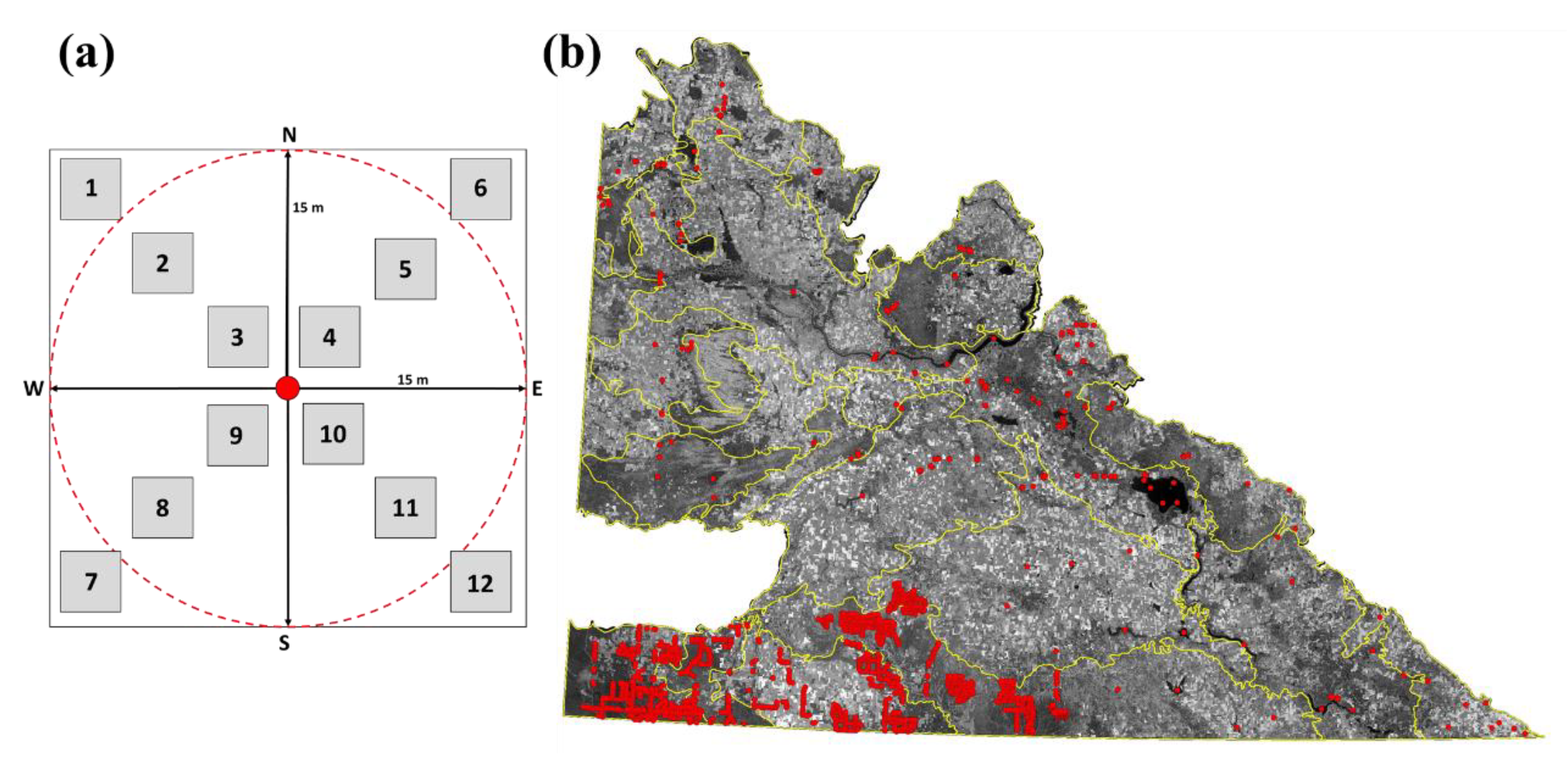
Ground-truthing is crucial in remote sensing-based classification research; the more precise field data, the more accurate the classification will be. This research depended on several intensive field surveys from 2016, 2017, 2018, and 2019 within all 25 landscape types in the MGE of Saskatchewan. In 2019, the field survey plots were designed to be commensurate with the remote sensing data properties such as the spatial coverage, pixel size, and temporal frequency (Figure 2a). Landcover identification technique was designed by the PLI team and grassland experts using 1 m2 quadrat over twelve (12) replicas from each survey plot of the year 2019’s field survey. The data cleansing process was conducted based on critical criteria such as edge effect, temporal landscape conditions, active location, wildfire, and floods. This stage required checking each point to determine whether it met the criteria above. The total number of the field survey used for this research was 2385, 30% of the samples were used for the training approach, and 70% were used for the testing (see Figure 2b).
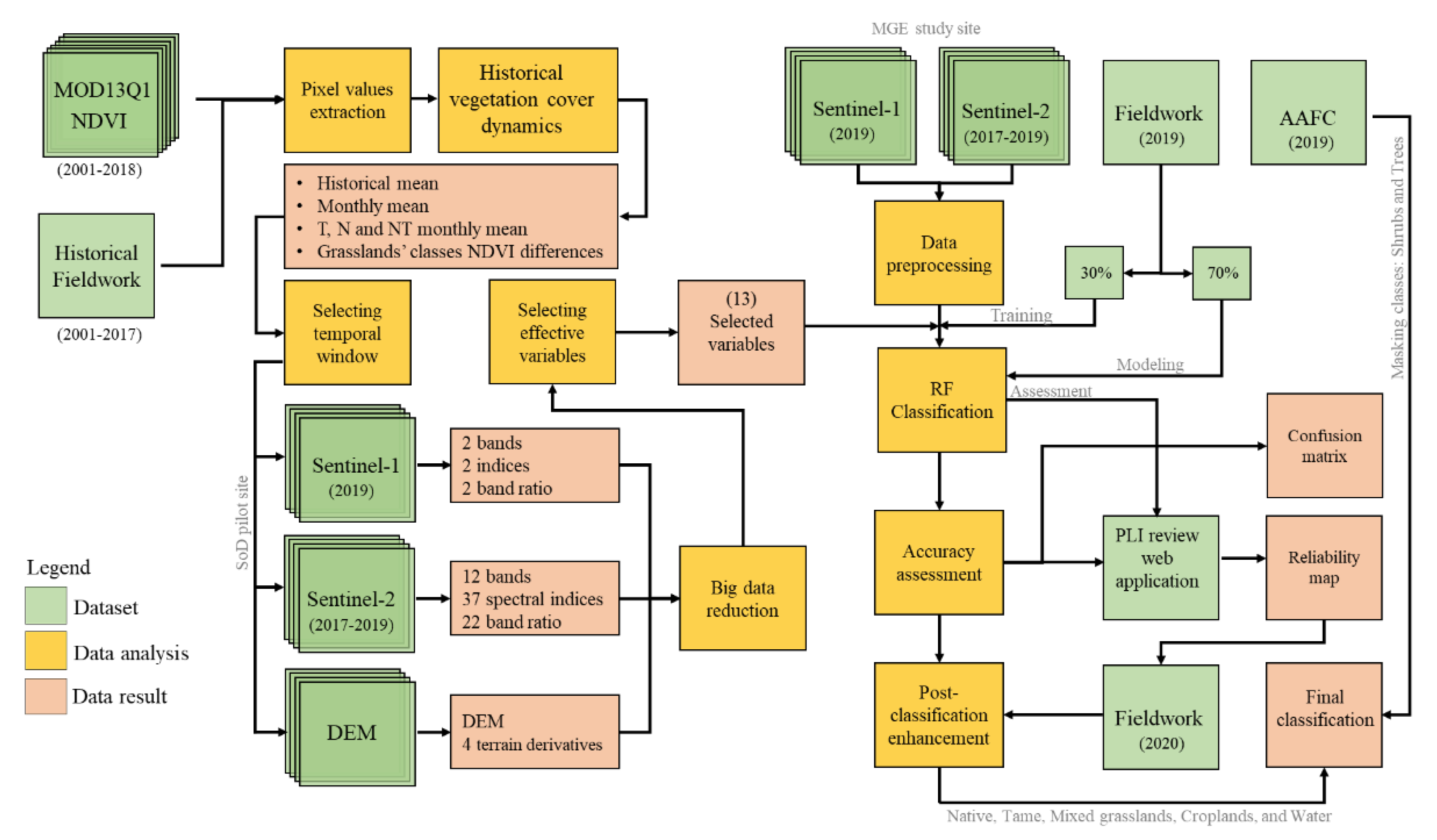
The University of Manitoba supercomputer was used to develop new techniques to handle big remote sensing reduction analyses. This research’s framework was built on the R programming language. Two scales of analysis were conducted; first, the temporal and spectral selection using time-series of low-resolution satellite data for a pilot site; second, ML analysis using high-resolution satellites (Figure 3).
3.2. Big Data Reduction
Selecting the best temporal window for data acquisition and knowing the most influential variables is vital information for subsequent modelling steps; it will support the modeling process, decrease the big data load, and improve classification accuracy. For that purpose, a smaller study area (14,157 km2) was chosen as a pilot site to understand the natural fluctuations of the vegetation cover in the MGE and test every possible variable that can be delivered from the available remote sensing datasets.
3.2.1. Temporal Window Selection
At this stage, 414 satellite images were obtained and analyzed to calculate the Normalized Difference Vegetation Index (NDVI) from the MOD13Q1, one of MOD13 series and Moderate Resolution Imaging Spectroradiometer (MODIS) satellite family. MOD13Q1 provides terrestrial photosynthetic vegetation cover with 16 days of temporal granularity with 250 m spatial resolution [28,29,30]. MODIStsp package is R package that processes MODIS data and analysis efficiently [31]. The overall monthly average of the pilot site and the monthly averages of the Native, Mixed, and Tame grassland classes identified from ground-truthing were calculated. Measuring the suitable time window for the satellite data acquisition has been done through the following equation:
where is the NDVI average of the month for the years 2001–2018 for the classes native, tame and mixed, and is the total absolute average for each month. The higher will be used as the base time for Sentinel-1 and Sentinel-2 data acquisition. The second filter is the availability of data with cloud coverage <5%, which is more applicable to Sentinel-2 as optical remote sensing.
3.2.2. Effective Variables Selection
R programming language was used to calculate 78 variables from Sentinel-1, Sentinel-2, and digital elevation model (DEM) datasets (see Table A1 in the Appendix A). A Principal Component Analysis (PCA) was used to implement the selection of the variables that cause higher variation within the native, tame, and mixed grassland classes. Petrovska et al. (2020) [32] found that PCA can be used as a data dimensionality reduction technique that can improve classification accuracy. This technique has been recently used to control big data complexity and sway prospective bias [33]. The principal components (PCs) that explained 90% of the total variance would be considered for the ML modeling [34].
3.3. Data Acquisition and Preprocessing
The MGE classification depended on two remote sensing sensors from the European Space Agency (ESA) under the Copernicus program. Sentinel-2 is the passive satellite sensor that uses the reflected solar radiation from the earth’s surface to create multispectral bands [35]; this satellite data is highly dependent on the atmospheric conditions and the cloud coverage [36,37]. And, the Sentinel-1 satellite as SAR, one of the active satellite sensors that produce and receive energy, is not affected by clouds or atmospheric conditions [38]. The obtained Sentinel-2 images were set to have minimum cloud coverage of <5% and were from 2017–2019. 25 tiles were selected for this research. getSpatialData R package was used for the data acquisition of Sentinel-1 and Sentinel-2 [39].
Sentinel Application Platform (SNAP) software was used to preprocess each band at each tile; these steps were conducted separately for Sentinel-1 and Sentinel-2 [38]. Filipponi (2019) proposed a workflow to perform the preprocessing to Sentinel-1 Ground Range Detected datasets. Seven major steps are needed for Sentinel-1 preprocessing; these steps were carried out based on [38] Filipponi (2019) recommendations, which are stated as (1) Apply Orbit File will be importing the precise orbit information such as the accurate satellite position and its velocity [38]; (2) Thermal Noise Removal operation will reduce the thermal noise effects through normalizing the backscattering signals; (3) Border Noise Removal to remove the low-intensity noise and scene’s edges [40]; (4) Calibration converts the pixels’ values to the radiometrically SAR backscattering values: (5) Speckle Filtering is an optional step, but it is important to increase image quality using Lee Sigma filter operator [41]; (6) Range Doppler Terrain Correction is intended to correct the geometrical distortion using DEM data available in SNAP, and (7) decibel (dB) conversion using logarithmic transformation. Sentinel-2 Multispectral Instrument (MSI) level-1C contained 13 spectral bands with 10, 20, and 60 m spatial resolutions [35,42]. This product has been radiometrically and geometrically corrected from level-1B using Sen2Cor [38]. Top of Atmosphere (TOA) reflectance conversion was computed for each band. The 25 tiles were reprojected to the case study Universal Transverse Mercator (UTM) projection zones. Mosaicking processes were conducted for each band to create the final layers for the calculation using PCI Geomatica software, and all mosaicked layers were resampled to 10 m pixel size to unify the data dimensions and pixels’ alignments.
3.4. Random Forest (RF) Classification
RFs are efficient machine learning algorithms for vegetation cover classification and typically provide higher prediction accuracy than other methods [29,43]. De’Ath and Fabricius (2000) concluded that a decision-based tree classification is a powerful tool for ecological research because of the following reasons: (1) flexibility to import a diverse data type; (2) ability to test the importance of many variables; (3) capability to assess modeling progress and strength; and (4) feasibility to generate reliable outputs in environmental research. The RF classifier is based on the generated decision trees from the aggregated bootstrapped training samples from ground-truthing [18,44], which was computed based on [45] steps, as follow:
where is the predicted pixel, = 1 to , is the aggregated bagged sample point for the training dataset, which is 30% of the total ground-truthing points.
The Gini Index is the classes-based measurement for the attribute selections which evaluate the importance of each used variable in the classification process [46], which is expressed mathematically as follow:
where is the training sample, and the is the probability that the selected case belongs to a class [46].
RF classification was conducted in the R language using coding packages (randomForest) and (randomForestExplainer); these two R packages helped understand variation caused by each variable, minimum depth of distribution, and identifying the interactions between variables; this tool aligned with Equations (2) and (3) [45]. The MGE’s grasslands were classified as a final step through ArcGIS Pro 2.6 Forest-based Classification and Regression tool. High vegetation canopy such as coniferous, deciduous, mixed forest, and shrubs were masked from the AAFC 2019 map; this approach was done to mitigate the impact of landscape diversity on the accuracy of the grassland’s classification. Additionally, a post classification comparison (PCC) technique was implemented between our classification and AAFCs 2017, 2018, and 2019 to assess classification consistency. We also used the pixel-based majority analysis with 3 × 3 and 5 × 5 kernel sizes in order to eliminate single unique pixel classes that have the potential of being misclassified.
3.5. Accuracy Assessment
The evaluation of the classification accuracy of this research used two types of assessments. The first assessment is the confusion matrix, which provides a summary in a cross-tabulation format between the classified classes and the ground-truthing data (Foody, 2002, 2010). This assessment included information on the overall accuracy (the total accurate prediction among all classified classes), the user’s accuracy (%), which represents the probability of a classified pixel into a given category that actually represents that category on the ground, and the producer’s accuracy (%) which represents how well reference pixels of the ground cover type are classified [18]. According to [47], Kappa indices failed to reflect and offer useful information on the classification accuracy because of the following two reasons: (1) it compares the accuracy to the baseline of randomness; and (2) it cannot deliver useful and fundamental information on the classification accuracy. Therefore, we decided not to use Kappa as an indicator of classification accuracy. Additionally, comparisons between our classification and other formal classifications will clarify the accuracy and the enhancement of our product as an addition to currently available Canadian landcover mapping products. The second assessment is the spatial distribution of errors; this type of assessment was implemented through the PLI Review Web Application. This application was designed specifically for this project and distributed to several grassland scientists and specialists in Saskatchewan to assess the classification accuracy of the map. This survey was built based on [48] previous research justifying classification reliability. The survey was constructed based on an ArcGIS Survey 123 application and asked participants to assess the quality of the classified map in relation to their knowledge of landcover on the ground at about 1521 survey points.
4. Results
4.1. Modeling Setup and Assessment Metrics
The preliminary data analysis of 17 years NDVI time-series for the pilot area showed normal fluctuations between the seasons and slight differences between the grassland classes. , and have the highest values in the period between 15 June to 15 August, which indicates that this period of the year is the optimum time window for obtaining remote sensing data for this research (Figure 4). The dimensionality reduction using PCA was effective and identified 20 variables explaining 90% of the variation between the classes. Secondly, the Pearson’s correlation matrices between the variables at each class confirmed a reduction in the number of the selected variables to ten raster layers: Normalized Difference Salinity Index (NDSI), Chlorophyll Red-Edge (Chlred-edge), Atmospherically Resistant Vegetation Index (ARVI), topographic wetness index (TWI), Sentinel-2 band12 divided by band2 (B12DB2), Sentinel-1 band VV divided by band VH (VVDVH), Sentinel-1 band VH divided by band VV (VHDVV), Sentinel-1 band VV subtracted by band VH (VVMVH), band VV, and band VH), see Figure A1 in the Appendix A.
The confusion matrix was used to compare the classified classes against the reference ground-truthing. Additionally, AAFC land cover maps for 2016, 2017, and 2018 were used in this assessment. Our classification has an overall accuracy of 90.2%, and AAFC has a 7–10% classification accuracy lower than ours. Cropland, Water, Tame classes have the highest Producer’s Accuracy as 97.21%, 95.16%, and 93.8%, respectively (Figure 5a). The native grassland 98.20% had user’s accuracy and 88.40% producer’s accuracy. The mixed grassland class has the lowest overall accuracy (82.83%) and very low user’s accuracy (45.8%); the AAFC maps of 2016, 2017, and 2018 have not provided this class which was noted in our research as non-classified data (NCD; Figure 5b–d). The second assessment approach using the PLI Review Web Application represents the experts’ opinion (nine professional ecologists at just over 1500 sites) which is another direction to discover and learn the strength and weaknesses of our prediction model; this assessment was conducted using only the native, tame, mixed, and cropland classes as they represent the dominant vegetation landscape classes in the case study. The average expert’s opinions (%) agreed with 73% for the Native class, 88% for the Tame class, 95% for the Mixed class, and 88% for the Cropland class (Figure 6).
4.2. Grassland Spatial Distribution
Native grassland occupies 33.9% (about 2.9 million hectares) of the MGE total area (8.63 million ha). Croplands are the dominant land cover class in the MGE, which covers 52.2% (4.5 million ha; Figure 7a). Tame grassland covered approximately 2.3% (about 0.2 million ha), and mixed grassland is 4% (0.34 million ha). It should be noted that this ecoregion likely has one of the highest proportions of native grassland remaining in Saskatchewan, whereas, in many other areas, grassland conversion has occurred at much higher rates. Water bodies in this ecoregion cover 5.5% (0.48 million ha). Shrubs and trees covered 1.5% (0.12 million ha) and 0.7% (0.06 million ha), respectively (see Figure 7b).
4.3. MGE’s Landscape-Based Grasslands
The MGE of Saskatchewan is divided into 25 landscape areas; each one of these landscapes has unique soil properties, topography, and soil organic matter. Wood Mountain Plateau landscape (886,679.55 ha) has the most native grassland area, 480,267.19 ha (54.2%); this portion is 16.5% of native grassland in MGE. Additionally, native grasslands cover 65.9% (81,848.13 ha) of the Great Sand Hills landscape area, 60.3% (160,204.94 ha) of Maple Creek Plain landscape, and 58.1% (79,134.53) of Old Man on His Back Plateau landscape. See Figure 8.
Mixed grassland is considered the modified grass introduced in the local ecosystem due to natural processes (e.g., wind blowing, surface water movement, and post-wildfire effects) or anthropogenic activities. Wild Horse Plain and Old Man on His Back Plateau landscapes have the highest mixed grasslands, 16.1% (41,516.27 ha) and 9.6% (13,109.45 ha), respectively.
Tame grassland is a vital forage for beef production in western Canada because of its higher above-ground biomass productivity in normal environmental conditions as compared to native grassland. 6.3% (16,754.48 ha) of Maple Creek Plain landscape area is inhabited by tame grassland and Beechy Hills landscape with 5.6% (16,014.75 ha).
Seven landscapes were found to be dominated by croplands, which are Sibbald Plain (70.5%), Eston Plain (70%), Antelope Creek Plain (69.2%), Swift Current Plateau (68.1), Kerrobert Plain (66.8%), Wood River Plain (66.5), and Lake Alma Upland (66.3%); these landscapes contributed about 53.5% (2.4 million ha) of the croplands in MGE.
5. Discussion
We are aware of only three other studies that have attempted to map and distinguish different grassland types in North America [5,49,50]. Only one of these studies occurred at a large spatial scale (5000 km2; [49]), and this study only used Landsat-based NDVI to distinguish two different grassland types. All three studies reported varying success at distinguishing native and tame grasslands, and none provided information on mixed grasslands. Our study also demonstrated a substantial improvement on the only available large-scale mapping products available for the agricultural region in Saskatchewan (AAFC). The mixed grassland class was found to have the lowest accuracy among other classes; Sentinel 2 images with 10 m spatial resolution might be the cause, and higher resolution satellite images such as RADARSAT-1 and RADARSAT-2 will improve the mixed grassland classification accuracy to above 90%, with respect to the quality and quantity of field survey and training datasets.
While many fields in Prairie Canada include some mixture of native and tame grasses and forbs either via deliberate planting, invasion, or reversion (fields that were tame but are reverting back to areas that are dominated by native species), ours is the first study that attempted to distinguish these grassland types (grasslands with >75% native or tame cover, and fields with some mixture of grassland vegetation). The other three studies we mention above [5,49,50] only distinguished predominately native or tame fields. While our study represents a significant step in classifying landcover in the prairies, we still came across significant difficulties distinguishing this particular mixed grassland landcover class. First, this landcover class was challenging to identify in the field and required significant expertise in botany to ground-truth. Second, the exact proportion of grassland types within a pixel likely has a significant impact on the spectral indices we used in our study (i.e., fields close to 75% will likely be distinguished more easily, whereas fields near equal mixtures will be harder to distinguish). It will likely be difficult in the future to identify this particular landcover class without higher resolution imagery (e.g., satellite or perhaps drone imagery) that can identify smaller patches of native and tame vegetation. However, even small areas (i.e., <1 m2) can still include a mixture of native and tame vegetation, which may make landcover classifications elusive in the future.
The native grassland result was found aligned with previous research findings, Gauthier and Wiken (2003) [9] reported that the native grassland remaining in the Saskatchewan MGE is 35.8%, and Hammermeister et al. (2001) [51] found that the native grassland is 31% and water is 5%. Our attempt at mapping prairie landcover demonstrated a large-scale assessment of grasslands in the Canadian Prairie over a 86,300 km2 region.
Sentinel 1 and 2 satellites provide exceptional opportunities, especially for mapping grasslands at high resolution in regional cases such as this; however, these opportunities also have prominent challenges [36]. And, the collective research opinion on how to overcome the challenges associated with big data in remote sensing research such as data management (e.g., radiometric enhancement, geometrical corrections, and mosaicking) and data modeling (e.g., spectral indices, time-series analysis, and classification) is to use strong analytical infrastructure (i.e., HPC and supper computers) and our research demonstrated this. A novel big data reduction technique was adopted in this research to reduce HPCs processing time and to improve the classification quality by filtering data through two factors, a temporal window that demonstrated significant differences between the grassland classes (i.e., native, tame and mixed), and a PCA technique which helped to shrink the data size and improve classification accuracy. The improvement of the accuracy did not depend on big remote sensing data only; rather accuracy increased when we integrated optical and SAR remote sensing and included this integration in the RF to identify each class.
6. Conclusions
In this research, an assessment of the current grassland spatial distribution was done using big remote sensing data from MODIS, Sentinel 1, and Sentinel 2. Numerous innovations were tackled in this regional research, comprising (i) understanding the optimum temporal window that is needed to conduct the field survey and the classification analysis for grassland mapping in the CP; this approach was proven in this study to improve the accuracy of the classification; (ii) integrating high-resolution passive and active remote sensing data to represent more comprehensively the soil-plant relationships within various landscapes and terrain topography; (iii) big geospatial data management through the data dimensionality reduction technique via PCA, this tactic reduced the number of raster variables from 78 to 10 (approximately, from 1620 GB to 200 GB), which is a reduction of about 87% of the original data load. This approach has a significant impact on the data modeling processing time from about one month for a single processing run to about one week; this saved time allowed us to focus more on the robustness of the classification algorithm; (iv) innovative assessment tool to understand the spatial distribution of the errors, and the classification assessment was built as a package to assess the reliability of the results from different perspectives: (1) diagnose the accuracy of the classification model, (2) compare the classification with the current AAFC classification, and (3) quantify the satisfaction of local ecologists and ranchers about how well the classification met their knowledge of landcover on the ground; and (4) improve the ground-truthing protocol through a consistent guideline that can be used in the future to update the classification.
This research demonstrated how machine learning algorithm such as Random Forest could be useful to generate valuable and accurate information on the spatial distribution of the grassland types (native, tame, and mixed) in the MGE of Saskatchewan. The MGE ecosystem is vulnerable to prolonged droughts, human disturbance, and over- or under-grazing. Therefore, building an effective environmental and agricultural policy that better mitigates these impacts is vital, which relies primarily on updated and accurate data such as the PLI classification. Moreover, these results will support the decision-makers of Saskatchewan to implement conservation plans to protect vulnerable ecosystems and species and implement site-specific management.
It is imperative to keep mapping the MGE every year or two to model the spatiotemporal dynamics of grassland landscapes. It will provide information to conservation ecologists about the spatiotemporal scales of grassland change, making decisions and actions more rapid, precise, and effective. This project can provide considerable support to the federal endeavor to map grassland in Canada with unified and comprehensive grassland definitions, sampling protocol, and learned lessons from PLI’s technical research in ML and big remote sensing data modeling.
Author Contributions
Conceptualization, N.B., B.P. and R.F.; methodology, N.B.; software, N.B. and R.F.; validation, N.B., B.P. and R.F.; formal analysis, N.B.; investigation, N.B., B.P. and R.F.; resources, N.B.; writing—original draft preparation, N.B.; writing—review and editing, N.B., B.P. and R.F.; visualization, N.B.; project administration, B.P. and R.F.; funding acquisition, B.P. and R.F. All authors have read and agreed to the published version of the manuscript.
Funding
This research was funded by the Government of Canada through the federal Department of Environment and Climate Change Canada, project number GCXE19C091.
Institutional Review Board Statement
Not applicable.
Informed Consent Statement
Not applicable.
Data Availability Statement
Not applicable.
Acknowledgments
Thanks to the numerous experts who assessed the accuracy of the final landcover mapping product: Chet Neufeld, Joseph Kotlar, Katherine Conkin, Maggi Sliwinski, Sarah Lee, and Sarah Ludlow. Thanks to Ben Sawa, Beryl Wait, and Sarah Vinge-Mazer for their valuable help in the fieldwork to assess and identify the grassland types. Additionally, Scott Watson and Andre Worms from the IT Services at the University of Manitoba for their help in HPC requests. And, special thanks to Mike Andersen, Xin Xia, and Ken Yurach for the technical support in the web applications. We would also like to thank various funding agencies that allowed us to complete this project: Environment and Climate Change Canada and Saskatchewan Ministry of Environment.
Conflicts of Interest
The authors declare no conflict of interest.
Appendix A

Table A1.
Description to the 78 raster-based variables used in ML classification for this research, including 13 Sentinel-2 bands; and 22 Sentinel-2 band ratios (; Bn is the band number), B3DB8, B3DB2, B10DB3, B10DB2, B4DB10, B4DB2, B5DB4, B5DB2, B11DB5, B11DB2, B6DB11, B6DB2, B7DB6, B8ADB7, B8ADB2, B12DB8A, B12DB2, B1DB12, B1DB2, B9DB1, B9DB2; 6 Sentinel-1 variables as 2 bands (VV and VH), 2 ratios (VV/VH and VH/VV) and 2 indices (VH-VV and VV-VH); 4 DEM variables (elevation, slope, Topographic Wetness Index (TWI) calculated as where A is the specific catchment area, and is the slope angle [51,52].
| Index | Name | Formula | Reference |
|---|---|---|---|
| NDVI | Normalized difference vegetation index | [53,54] | |
| SAVI | Soil-adjusted vegetation index | [55] | |
| GNDVI | Green Normalized Difference Vegetation Index | [56] | |
| MCARI | Modified Chlorophyll Absorption in Reflectance Index | [56] | |
| PVI | Perpendicular Vegetation Index | [57] | |
| IRECI | The Inverted Red-Edge Chlorophyll Index | [58] | |
| S2REP | The Sentinel-2 Red-Edge Position Index | [59] | |
| MTCI | The Meris Terrestrial Chlorophyll Index | [60] | |
| ARVI | The Atmospherically Resistant Vegetation Index | [61] | |
| EVI | Enhanced Vegetation Index | [62] | |
| EVI-2 | Enhanced Vegetation Index 2 | [63] | |
| Chlred-edge | Chlorophyll Red-Edge | [64] | |
| EPI | EPI | [65] | |
| IVI | Ideal vegetation index | [66] | |
| LCI | Leaf Chlorophyll Index | [67,68] | |
| GVI | Tasselled Cap-vegetation | [69,70,71] | |
| WDRVI | Wide Dynamic Range Vegetation Index | [72,73] | |
| SLAVI | Specific Leaf Area Vegetation Index | [74] | |
| SIPI3 | Structure Intensive Pigment Index 3 | [68,75] | |
| YVIMSS | Tasselled Cap-Yellow Vegetation Index MSS | [70,76] | |
| NDII | Normalized Difference 819/1600 | [77,78] | |
| PNDVI | Pan NDVI | [79] | |
| RDVI | RDVI | [80] | |
| SCI | Soil Composition Index | [81] | |
| MSBI | Misra Soil Brightness Index | [82] | |
| BI2 | The second Brightness Index algorithm | [83] | |
| BI | The Brightness Index algorithm | [84] | |
| SBL | Soil Background Line | [57] | |
| NDSI | Normalized Difference Salinity Index | [81] | |
| MNDWI | the Modified Normalized Difference Water Index (MDNWI) | [85] | |
| NDWI | normalized difference water index | [86] | |
| NDWI2 | The second Normalized Difference Water Index algorithm | [85] | |
| NDPI | The Normalized Difference Pond Index | [87] |
Figure A1.
Person correlations between 10 raster-based variables derived from Sentinel-1 and Sentinel-2 for different land cover classes in the SoD (pilot site).
Figure A1.
Person correlations between 10 raster-based variables derived from Sentinel-1 and Sentinel-2 for different land cover classes in the SoD (pilot site).

References
- Thorpe, J.; Wolfe, S.A.; Houston, B. Potential Impacts of Climate Change on Grazing Capacity of Native Grasslands in the Canadian Prairies. Can. J. Soil Sci. 2008, 88, 595–609. [Google Scholar] [CrossRef]
- Gauthier, D.A.; Wiken, E.D.B. Monitoring the Conservation of Grassland Habitats, Prairie Ecozone, Canada. Environ. Monit. Assess. 2003, 88, 343–364. [Google Scholar] [CrossRef]
- Hoekstra, J.M.; Boucher, T.M.; Ricketts, T.H.; Roberts, C. Confronting a Biome Crisis: Global Disparities of Habitat Loss and Protection. Ecol. Lett. 2004, 8, 23–29. [Google Scholar] [CrossRef]
- Stephens, S.E.; Walker, J.A.; Blunck, D.R.; Jayaraman, A.; Naugle, D.E.; Ringelman, J.K.; Smith, A.J. Predicting Risk of Habitat Conversion in Native Temperate Grasslands. Conserv. Biol. 2008, 22, 1320–1330. [Google Scholar] [CrossRef]
- Fisher, R.J.; Sawa, B.; Prieto, B. A Novel Technique Using LiDAR to Identify Native-Dominated and Tame-Dominated Grasslands in Canada. Remote Sens. Environ. 2018, 218, 201–206. [Google Scholar] [CrossRef]
- Brooks, T.M.; Mittermeier, R.A.; Mittermeier, C.G.; da Fonseca, G.A.B.; Rylands, A.B.; Konstant, W.R.; Flick, P.; Pilgrim, J.; Oldfield, S.; Magin, G.; et al. Habitat Loss and Extinction in the Hotspots of Biodiversity. Conserv. Biol. 2002, 16, 909–923. [Google Scholar] [CrossRef] [Green Version]
- Looman, J. Preliminary Classification of Grasslands in Saskatchewan. Ecology 1963, 44, 15–29. [Google Scholar] [CrossRef]
- Coupland, R.T.; Brayshaw, T.C. The Fescue Grassland in Saskatchewan. Ecology 1953, 34, 386–405. [Google Scholar] [CrossRef]
- Amichev, B.Y.; Bentham, M.J.; Kulshreshtha, S.N.; Laroque, C.P.; Piwowar, J.M.; van Rees, K.C.J. Carbon Sequestration and Growth of Six Common Tree and Shrub Shelterbelts in Saskatchewan, Canada. Can. J. Soil Sci. 2016, 97, 368–381. [Google Scholar] [CrossRef]
- Hammermeister, A.; Gauthier, D.; McGovern, K. Saskatchewan’s Native Prairie: Statistics of a Vanishing Ecosystem and Dwindling Resource; Native Plant Society of Saskatchewan Inc.: Saskatoon, SK, Canada, 2001. [Google Scholar]
- Fisette, T.; Rollin, P.; Aly, Z.; Campbell, L.; Daneshfar, B.; Filyer, P.; Smith, A.; Davidson, A.; Shang, J.; Jarvis, I. AAFC Annual Crop Inventory: Status and Challenges. In Proceedings of the Second International Conference on Agro-Geoinformatics (Agro-Geoinformatics), Fairfax, VA, USA, 12–16 August 2013; pp. 270–274. [Google Scholar] [CrossRef]
- Ali, I.; Cawkwell, F.; Dwyer, E.; Barrett, B.; Green, S. Satellite Remote Sensing of Grasslands: From Observation to Management. J. Plant Ecol. 2016, 9, 649–671. [Google Scholar] [CrossRef] [Green Version]
- Badreldin, N.; Xing, Z.; Goossens, R. The Application of Satellite-Based Model and Bi-Stable Ecosystem Balance Concept to Monitor Desertification in Arid Lands, a Case Study of Sinai Peninsula. Modeling Earth Syst. Environ. 2017, 3, 21. [Google Scholar] [CrossRef]
- Reinke, K.; Jones, S. Integrating Vegetation Field Surveys with Remotely Sensed Data. Ecol. Manag. Restor. 2006, 7, S18–S23. [Google Scholar] [CrossRef]
- Xie, Y.; Sha, Z.; Yu, M. Remote Sensing Imagery in Vegetation Mapping: A Review. J. Plant Ecol. 2008, 1, 9–23. [Google Scholar] [CrossRef]
- Kolecka, N.; Ginzler, C.; Pazur, R.; Price, B.; Verburg, P. Regional Scale Mapping of Grassland Mowing Frequency with Sentinel-2 Time Series. Remote Sens. 2018, 10, 1221. [Google Scholar] [CrossRef] [Green Version]
- Li, S.; Dragicevic, S.; Castro, F.A.; Sester, M.; Winter, S.; Coltekin, A.; Pettit, C.; Jiang, B.; Haworth, J.; Stein, A.; et al. Geospatial Big Data Handling Theory and Methods: A Review and Research Challenges. ISPRS J. Photogramm. Remote Sens. 2016, 115, 119–133. [Google Scholar] [CrossRef] [Green Version]
- Badreldin, N.; Abu Hatab, A.; Lagerkvist, C.J. Spatiotemporal Dynamics of Urbanization and Cropland in the Nile Delta of Egypt Using Machine Learning and Satellite Big Data: Implications for Sustainable Development. Environ. Monit. Assess. 2019, 191, 767. [Google Scholar] [CrossRef]
- Laney, D. Data Management: Controlling Data Volume, Velocity, and Variety. Appl. Deliv. Strateg. 2001, 6, 6. [Google Scholar]
- Suthaharan, S. Big Data Classification: Problems and Challenges in Network Intrusion Prediction with Machine Learning. ACM SIGMETRICS Perform. Eval. Rev. 2014, 41, 70–73. [Google Scholar] [CrossRef]
- Hogland, J.; Anderson, N. Function Modeling Improves the Efficiency of Spatial Modeling Using Big Data from Remote Sensing. Big Data Cogn. Comput. 2017, 1, 3. [Google Scholar] [CrossRef] [Green Version]
- Mahdianpari, M.; Salehi, B.; Mohammadimanesh, F.; Brisco, B.; Homayouni, S.; Gill, E.; DeLancey, E.R.; Bourgeau-Chavez, L. Big Data for a Big Country: The First Generation of Canadian Wetland Inventory Map at a Spatial Resolution of 10-m Using Sentinel-1 and Sentinel-2 Data on the Google Earth Engine Cloud Computing Platform. Can. J. Remote Sens. 2020, 46, 15–33. [Google Scholar] [CrossRef]
- Acton, D.F.; Padbury, G.A.; Stushnoff, C.T. The Ecoregions of Saskatchewan; Saskatchewan Environment and Resource Management, Canadian Plains Research Center: Regina, SK, USA, 1998. [Google Scholar]
- Gauthier, D.A.; Patino, L.; McGovern, K. Status of Native Prairie Habitat, Prairie Ecozone, Saskatchewan; Project Report to Wildlife Habitat Canada, Number 8.65A.1R-01/02; Canadian Plains Research Centre: Regina, SK, USA, 2002; 355p. [Google Scholar]
- Janzen, H.H.; Campbell, C.A.; Izaurralde, R.C.; Ellert, B.H.; Juma, N.; McGill, W.B.; Zentner, R.P. Management Effects on Soil C Storage on the Canadian Prairies. Soil Tillage Res. 1998, 47, 181–195. [Google Scholar] [CrossRef]
- Thomas, A.F.; Thomas, E.B.; Chris, H.H. Successes of Soil Conservation in the Canadian Prairies Highlighted by a Historical Decline in Blowing Dust. Environ. Res. Lett. 2012, 7, 14008. [Google Scholar] [CrossRef]
- Bai, Y.; Abouguendia, Z.; Redmann, R.E. Relationship between Plant Species Diversity and Grassland Condition. Rangel. Ecol. Manag. /J. Range Manag. Arch. 2001, 54, 177–183. [Google Scholar]
- Didan, K. MOD13Q1 MODIS/Terra Vegetation Indices 16-Day L3 Global 1km SIN Grid V006; NASA EOSDIS LP DAAC: Sioux Falls, SD, USA, 2015. [Google Scholar] [CrossRef]
- Nitze, I.; Barrett, B.; Cawkwell, F. Temporal Optimisation of Image Acquisition for Land Cover Classification with Random Forest and MODIS Time-Series. Int. J. Appl. Earth Obs. Geoinf. 2015, 34, 136–146. [Google Scholar] [CrossRef] [Green Version]
- Didan, K.; Barreto Munoz, A.; Solano, R.; Huete, A. MODIS Vegetation Index User’s Guide (MOD13 Series); Vegetation Index and Phenology Lab, University of Arizona: Tucson, AZ, USA, 2015. [Google Scholar]
- Busetto, L.; Ranghetti, L. MODIStsp: An R Package for Automatic Preprocessing of MODIS Land Products Time Series. Comput. Geosci. 2016, 97, 40–48. [Google Scholar] [CrossRef] [Green Version]
- Petrovska, B.; Zdravevski, E.; Lameski, P.; Corizzo, R.; Štajduhar, I.; Lerga, J. Deep Learning for Feature Extraction in Remote Sensing: A Case-Study of Aerial Scene Classification. Sensors 2020, 20, 3906. [Google Scholar] [CrossRef] [PubMed]
- Clark, J.; Provost, F. Unsupervised Dimensionality Reduction versus Supervised Regularization for Classification from Sparse Data. Data Min. Knowl. Discov. 2019, 33, 871–916. [Google Scholar] [CrossRef] [Green Version]
- Khaled, A.Y.; Abd Aziz, S.; Khairunniza Bejo, S.; Mat Nawi, N.; Jamaludin, D.; Ibrahim, N.U.A. A Comparative Study on Dimensionality Reduction of Dielectric Spectral Data for the Classification of Basal Stem Rot (BSR) Disease in Oil Palm. Comput. Electron. Agric. 2020, 170, 105288. [Google Scholar] [CrossRef]
- Drusch, M.; del Bello, U.; Carlier, S.; Colin, O.; Fernandez, V.; Gascon, F.; Hoersch, B.; Isola, C.; Laberinti, P.; Martimort, P.; et al. Sentinel-2: ESA’s Optical High-Resolution Mission for GMES Operational Services. Remote Sens. Environ. 2012, 120, 25–36. [Google Scholar] [CrossRef]
- Clerici, N.; Valbuena Calderón, C.A.; Posada, J.M. Fusion of Sentinel-1a and Sentinel-2A Data for Land Cover Mapping: A Case Study in the Lower Magdalena Region, Colombia. J. Maps 2017, 13, 718–726. [Google Scholar] [CrossRef] [Green Version]
- De Keukelaere, L.; Sterckx, S.; Adriaensen, S.; Knaeps, E.; Reusen, I.; Giardino, C.; Bresciani, M.; Hunter, P.; Neil, C.; van der Zande, D.; et al. Atmospheric Correction of Landsat-8/OLI and Sentinel-2/MSI Data Using ICOR Algorithm: Validation for Coastal and Inland Waters. Eur. J. Remote Sens. 2018, 51, 525–542. [Google Scholar] [CrossRef] [Green Version]
- Filipponi, F. Sentinel-1 GRD Preprocessing Workflow. Proceedings 2019, 18, 11. [Google Scholar] [CrossRef] [Green Version]
- Kwok, R. Ecology’s Remote-Sensing Revolution. Nature 2018, 556, 137–138. [Google Scholar] [CrossRef] [PubMed]
- Hajduch, G. Masking “No-Value” Pixels on GRD Products Generated by the Sentinel-1 ESA IPF; European Space Agency (ESA): Ramonville Saint-Agne, France, 2018. [Google Scholar]
- Lee, J.S.; Jurkevich, I.; Dewaele, P.; Wambacq, P.; Oosterlinck, A. Speckle Filtering of Synthetic Aperture Radar Images: A Review. Remote Sens. Rev. 1994, 8, 313–340. [Google Scholar] [CrossRef]
- Roy, D.P.; Li, J.; Zhang, H.K.; Yan, L. Best Practices for the Reprojection and Resampling of Sentinel-2 Multi Spectral Instrument Level 1C Data. Remote Sens. Lett. 2016, 7, 1023–1032. [Google Scholar] [CrossRef]
- De’Ath, G.; Fabricius, K.E. Classification and Regression Trees: A Powerful yet Simple Technique for Ecological Data Analysis. Ecology 2000, 81, 3178–3192. [Google Scholar] [CrossRef]
- Liaw, A.; Wiener, M. Breiman and Cutler’s Random Forests for Classification and Regression. The Comprehensive R Archive Network (CRAN). 2018. Volume 29. Available online: http://math.furman.edu/~dcs/courses/math47/R/library/randomForest/html/00Index.html (accessed on 1 December 2021).
- Breiman, L. Random Forests. Mach. Learn. 2001, 45, 5–32. [Google Scholar] [CrossRef] [Green Version]
- Pal, M. Random Forest Classifier for Remote Sensing Classification. Int. J. Remote Sens. 2005, 26, 217–222. [Google Scholar] [CrossRef]
- Pontius, R.G.; Millones, M. Death to Kappa: Birth of Quantity Disagreement and Allocation Disagreement for Accuracy Assessment. Int. J. Remote Sens. 2011, 32, 4407–4429. [Google Scholar] [CrossRef]
- Foody, G.M. Explaining the Unsuitability of the Kappa Coefficient in the Assessment and Comparison of the Accuracy of Thematic Maps Obtained by Image Classification. Remote Sens. Environ. 2020, 239, 111630. [Google Scholar] [CrossRef]
- Olimb, S.K.; Dixon, A.P.; Dolfi, E.; Engstrom, R.; Anderson, K. Prairie or Planted? Using Time-Series NDVI to Determine Grassland Characteristics in Montana. GeoJournal 2017, 83, 819–834. [Google Scholar] [CrossRef]
- McInnes, W.S.; Smith, B.; McDermid, G.J. Discriminating Native and Nonnative Grasses in the Dry Mixedgrass Prairie with MODIS NDVI Time Series. IEEE J. Sel. Top. Appl. Earth Obs. Remote Sens. 2015, 8, 1395–1403. [Google Scholar] [CrossRef]
- Hickey, R. Slope Angle and Slope Length Solutions for GIS. Cartography 2000, 29, 1–8. [Google Scholar] [CrossRef]
- Mattivi, P.; Franci, F.; Lambertini, A.; Bitelli, G. TWI Computation: A Comparison of Different Open Source GISs. Open Geospat. Data Softw. Stand. 2019, 4, 1–12. [Google Scholar] [CrossRef]
- Tucker, C.J. Red and Photographic Infrared Linear Combinations for Monitoring Vegetation. Remote Sens. Environ. 1979, 8, 127–150. [Google Scholar] [CrossRef] [Green Version]
- Sellers, P.J. Canopy Reflectance, Photosynthesis and Transpiration. Int. J. Remote Sens. 1985, 6, 1335–1372. [Google Scholar] [CrossRef]
- Huete, A.R. A Soil-Adjusted Vegetation Index (SAVI). Remote Sens. Environ. 1988, 25, 295–309. [Google Scholar] [CrossRef]
- Daughtry, C.S.T.; Walthall, C.L.; Kim, M.S.; de Colstoun, E.B.; McMurtrey, J.E. Estimating Corn Leaf Chlorophyll Concentration from Leaf and Canopy Reflectance. Remote Sens. Environ. 2000, 74, 229–239. [Google Scholar] [CrossRef]
- Richardson, A.J.; Wiegand, C.L. Distinguishing Vegetation from Soil Background Information. Photogramm. Eng. Remote Sens. 1977, 43, 1541–1552. [Google Scholar]
- Clevers, J.G.P.W.; De Jong, S.M.; Epema, G.F.; Addink, E.A. MERIS and The Red-Edge Index. In Proceedings of the Second EARSeL Workshop on Imaging Spectroscopy; Springer: Enschede, The Netherlands, 2000; p. 14. [Google Scholar]
- Guyot, G.; Baret, F. Utilisation de la haute resolution spectrale pour suivre l’etat des couverts vegetaux. In Proceedings of the 4th International Colloquium on Spectral Signatures of Objects in Remote Sensing, Aussois, France, 12–18 January 1988; pp. 279–286. [Google Scholar]
- Dash, J.; Curran, P.J. Evaluation of the MERIS Terrestrial Chlorophyll Index (MTCI). Adv. Space Res. 2007, 39, 100–104. [Google Scholar] [CrossRef]
- Kaufman, Y.J.; Tanre, D. Atmospherically Resistant Vegetation Index (ARVI) for EOS-MODIS. IEEE Trans. Geosci. Remote Sens. 1992, 30, 261–270. [Google Scholar] [CrossRef]
- Huete, A.R.; Justice, C.; van Leeuwen, W. MODIS Vegetation Index (MOD13); Algorithm Theoretical Basis Document (ATBD); Department of Environmental Sciences, University of Virginia: Tucson, AZ, USA, 1999. [Google Scholar]
- Miura, T.; Yoshioka, H.; Fujiwara, K.; Yamamoto, H. Inter-Comparison of ASTER and MODIS Surface Reflectance and Vegetation Index Products for Synergistic Applications to Natural Resource Monitoring. Sensors 2008, 8, 2480–2499. [Google Scholar] [CrossRef] [Green Version]
- Gitelson, A.A.; Keydan, G.P.; Merzlyak, M.N. Three-Band Model for Noninvasive Estimation of Chlorophyll, Carotenoids, and Anthocyanin Contents in Higher Plant Leaves. Geophys. Res. Lett. 2006, 33, L11402. [Google Scholar] [CrossRef] [Green Version]
- Datt, B. Remote Sensing of Chlorophyll a, Chlorophyll b, Chlorophyll A+b, and Total Carotenoid Content in Eucalyptus Leaves. Remote Sens. Environ. 1998, 66, 111–121. [Google Scholar] [CrossRef]
- Baret, F.; Guyot, G.; Major, D. TSAVI: A Vegetation Index Which Minimizes Soil Brightness Effects on LAI and APAR Estimation. In Proceedings of the 12th Canadian Symposium on Remote Sensing and IGARSS’89, Vancouver, BC, Canada, 10–14 July 1989; pp. 1355–1358. [Google Scholar]
- Datt, B. Remote Sensing of Water Content in Eucalyptus Leaves. Aust. J. Bot. 1999, 47, 909. [Google Scholar] [CrossRef]
- Pu, R.; Gong, P.; Yu, Q. Comparative Analysis of EO-1 ALI and Hyperion, and Landsat ETM+ Data for Mapping Forest Crown Closure and Leaf Area Index. Sensors 2008, 8, 3744–3766. [Google Scholar] [CrossRef] [Green Version]
- Crist, E.P.; Cicone, R.C. A Physically-Based Transformation of Thematic Mapper Data—The TM Tasseled Cap. IEEE Trans. Geosci. Remote Sens. 1984, GE-22, 256–263. [Google Scholar] [CrossRef]
- Bannari, A.; Morin, D.; Bonn, F.; Huete, A.R. A Review of Vegetation Indices. Remote Sens. Rev. 1995, 13, 95–120. [Google Scholar] [CrossRef]
- Ferencz, C.; Bognár, P.; Lichtenberger, J.; Hamar, D.; Tarcsai, G.; Timár, G.; Molnár, G.; Pásztor, S.Z.; Steinbach, P.; Székely, B.; et al. Crop Yield Estimation by Satellite Remote Sensing. Int. J. Remote Sens. 2004, 25, 4113–4149. [Google Scholar] [CrossRef]
- Gitelson, A.A. Wide Dynamic Range Vegetation Index for Remote Quantification of Biophysical Characteristics of Vegetation. J. Plant Physiol. 2004, 161, 165–173. [Google Scholar] [CrossRef] [Green Version]
- Hancock, D.W.; Dougherty, C.T. Relationships between Blue- and Red-Based Vegetation Indices and Leaf Area and Yield of Alfalfa. Crop Sci. 2007, 47, 2547. [Google Scholar] [CrossRef]
- Lymburne, L.; Beggs, P.J.; Jacobson, C.R. Estimation of Canopy-Average Surface-Specific Leaf Area Using Landsat TM Data. Photogramm. Eng. Remote Sens. 2000, 66, 183–191. [Google Scholar]
- Blackburn, G.A. Spectral Indices for Estimating Photosynthetic Pigment Concentrations: A Test Using Senescent Tree Leaves. Int. J. Remote Sens. 1998, 19, 657–675. [Google Scholar] [CrossRef]
- Kauth, R.; Thomas, G. The Tasselled Cap—A Graphic Description of the Spectral-Temporal Development of Agricultural Crops as Seen by LANDSAT. In Symposium on Machine Processing of Remotely Sensed Data; The Laboratory for Applications of Remote Sensing, Purdue University: West Lafayette, IN, USA, 1976; pp. 41–51. [Google Scholar]
- Hardinsky, M.A.; Lemas, V. The Influence of Soil Salinity, Growth Form, and Leaf Moisture on the Spectral Reflectance of Spartina Alternifolia Canopies. Photogramm. Eng. Remote Sens. 1983, 49, 77–83. [Google Scholar]
- Le Maire, G.; François, C.; Soudani, K.; Berveiller, D.; Pontailler, J.-Y.; Bréda, N.; Genet, H.; Davi, H.; Dufrêne, E. Calibration and Validation of Hyperspectral Indices for the Estimation of Broadleaved Forest Leaf Chlorophyll Content, Leaf Mass per Area, Leaf Area Index and Leaf Canopy Biomass. Remote Sens. Environ. 2008, 112, 3846–3864. [Google Scholar] [CrossRef]
- Wang, F.; Huang, J.; Tang, Y.; Wang, X. New Vegetation Index and Its Application in Estimating Leaf Area Index of Rice. Rice Sci. 2007, 14, 195–203. [Google Scholar] [CrossRef]
- Broge, N.H.; Leblanc, E. Comparing Prediction Power and Stability of Broadband and Hyperspectral Vegetation Indices for Estimation of Green Leaf Area Index and Canopy Chlorophyll Density. Remote Sens. Environ. 2001, 76, 156–172. [Google Scholar] [CrossRef]
- Al-Khaier, F. Soil Salinity Detection Using Satellite Remote Sensing. Master’s Thesis, Universiteit Twenten, Enschede, The Netherlands, 2003. [Google Scholar]
- Misra, P.N.; Wheeler, S.G.; Oliver, R.E. Kauth-Thomas Brightness and Greenness Axes; NASA: Washington, DC, USA, 1977; pp. 23–46. [Google Scholar]
- Gadal, S.; Ouerghemmi, W.; Gadal, S.; Ouerghemmi, W. Multi-Level Morphometric Characterization of Built-up Areas and Change Detection in Siberian Sub-Arctic Urban Area: Yakutsk. ISPRS Int. J. Geo-Inf. 2019, 8, 129. [Google Scholar] [CrossRef] [Green Version]
- Schmidt, H.; Karnieli, A. Sensitivity of Vegetation Indices to Substrate Brightness in Hyper-Arid Environment: The Makhtesh Ramon Crater (Israel) Case Study. Int. J. Remote Sens. 2001, 22, 3503–3520. [Google Scholar] [CrossRef]
- Xu, H. Modification of Normalised Difference Water Index (NDWI) to Enhance Open Water Features in Remotely Sensed Imagery. Int. J. Remote Sens. 2006, 27, 3025–3033. [Google Scholar] [CrossRef]
- Gao, B. NDWI—A Normalized Difference Water Index for Remote Sensing of Vegetation Liquid Water from Space. Remote Sens. Environ. 1996, 58, 257–266. [Google Scholar] [CrossRef]
- Lacaux, J.P.; Tourre, Y.M.; Vignolles, C.; Ndione, J.A.; Lafaye, M. Classification of Ponds from High-Spatial Resolution Remote Sensing: Application to Rift Valley Fever Epidemics in Senegal. Remote Sens. Environ. 2007, 106, 66–74. [Google Scholar] [CrossRef]
Figure 1.
The geographical location of the case study (MGE) in Saskatchewan and landscape areas (M#); M1 Kerrobert Plain; M2 Sibbald Plain; M3 Oyen Upland; M4 Eston Plain; M5 Bad Hills; M6 Acadia Valley Plain; M7 Bindloss Plain; M8 Hazlet Plain; M9 Schuler Plain; Maple Creek Plain; M11 Great Sand Hills; M12 Antelope Creek Plain; M13 Gull Lake Plain; M14 Beechy Hills; M15 Coteau Hills; M16 Chaplin Plain; M17 Swift Current Plateau; M18 Wood River Plain; M19 Dirt Hills; M20 Coteau Lakes Upland; M21 Lake Alma Upland; M22 Wood Mountain Plateau; M23 Climax Plain; M24 Wild Horse Plain; M25 Old Man on His Back Plateau.

Figure 2.
The ground-truthing of PLI during the survey year 2019 and historical field survey data; (a) the survey plot designed for grassland identification survey in 2019; (b) the field survey spatial coverage (n = 2385) from several PLI field surveys and historical filtered databases.
Figure 2.
The ground-truthing of PLI during the survey year 2019 and historical field survey data; (a) the survey plot designed for grassland identification survey in 2019; (b) the field survey spatial coverage (n = 2385) from several PLI field surveys and historical filtered databases.

Figure 3.
The overall workflow of MGE mapping procedures using various remote sensing datasets and platforms to produce PLI MGE classification for 2019.
Figure 3.
The overall workflow of MGE mapping procedures using various remote sensing datasets and platforms to produce PLI MGE classification for 2019.

Figure 4.
The monthly averages of 17 years NDVI of differences between native and tame grasslands , differences between native and mixed grasslands and differences between tame and mixed grasslands .
Figure 4.
The monthly averages of 17 years NDVI of differences between native and tame grasslands , differences between native and mixed grasslands and differences between tame and mixed grasslands .

Figure 5.
The accuracy assessment of the MGE classification, User’s Accuracy (%): This value represents the probability of a classified pixel into a given category represents that category on the ground, and the Producer’s Accuracy (%): This value represents how well reference pixels of the ground cover type are classified; (a) PLI classification; (b) AAFC 2017; (c) AAFC 2018; and (d) AAFC 2019.

Figure 6.
Quantification of the accuracy assessment depending on local ecologists using a spatial survey web portal (PLI Review Web Application) to calculate opinion of MGE classification.
Figure 6.
Quantification of the accuracy assessment depending on local ecologists using a spatial survey web portal (PLI Review Web Application) to calculate opinion of MGE classification.

Figure 7.
The MGE classification of 2019; (a) The spatial distribution of the MGE grasslands classification; (b) the percentages (%) of classes areas in the MGE of Saskatchewan.
Figure 7.
The MGE classification of 2019; (a) The spatial distribution of the MGE grasslands classification; (b) the percentages (%) of classes areas in the MGE of Saskatchewan.

Figure 8.
The shared area percentages (%) of PLI classes over the 25 landscape areas in the MGE of Saskatchewan.
Figure 8.
The shared area percentages (%) of PLI classes over the 25 landscape areas in the MGE of Saskatchewan.

Table 1.
The definitions of the classes that were chosen in the PLI project for field survey and mapping.
Table 1.
The definitions of the classes that were chosen in the PLI project for field survey and mapping.
| Class | Definition |
|---|---|
| Native | This class represents the native grassland, composed primarily (>75%) of native grass species, such as:
|
| Mixed | This class represents one or more of the followings cases:
|
| Tame | This class represents the tame grassland areas that have, in most cases, been intentionally modified and are composed primarily (>75%) of planted introduced grasses and forbs such as:
|
| Cropland | This class represents all annually cultivated areas and summer-fallow crops. |
| Shrub | This class represents the predominantly woody vegetation of relatively low height (generally <2 m). |
| Forest | This class represents the predominantly forest areas such as:
|
| Water | This class represents deep water bodies such as lakes and rivers and shallow water bodies
|
Publisher’s Note: MDPI stays neutral with regard to jurisdictional claims in published maps and institutional affiliations. |
© 2021 by the authors. Licensee MDPI, Basel, Switzerland. This article is an open access article distributed under the terms and conditions of the Creative Commons Attribution (CC BY) license (https://creativecommons.org/licenses/by/4.0/).
Share and Cite
MDPI and ACS Style
Badreldin, N.; Prieto, B.; Fisher, R. Mapping Grasslands in Mixed Grassland Ecoregion of Saskatchewan Using Big Remote Sensing Data and Machine Learning. Remote Sens. 2021, 13, 4972. https://doi.org/10.3390/rs13244972
AMA Style
Badreldin N, Prieto B, Fisher R. Mapping Grasslands in Mixed Grassland Ecoregion of Saskatchewan Using Big Remote Sensing Data and Machine Learning. Remote Sensing. 2021; 13(24):4972. https://doi.org/10.3390/rs13244972
Chicago/Turabian StyleBadreldin, Nasem, Beatriz Prieto, and Ryan Fisher. 2021. "Mapping Grasslands in Mixed Grassland Ecoregion of Saskatchewan Using Big Remote Sensing Data and Machine Learning" Remote Sensing 13, no. 24: 4972. https://doi.org/10.3390/rs13244972
Note that from the first issue of 2016, this journal uses article numbers instead of page numbers. See further details here.