


Abstract
TRAPPIST-1 is a nearby system of seven Earth-sized, temperate, rocky exoplanets transiting a Jupiter-sized M8.5V star, ideally suited for in-depth atmospheric studies. Each TRAPPIST-1 planet has been observed in transmission both from space and from the ground, confidently rejecting cloud-free, hydrogen-rich atmospheres. Secondary eclipse observations of TRAPPIST-1 b with JWST/MIRI are consistent with little to no atmosphere given the lack of heat redistribution. Here we present the first transmission spectra of TRAPPIST-1 b obtained with JWST/NIRISS over two visits. The two transmission spectra show moderate to strong evidence of contamination from unocculted stellar heterogeneities, which dominates the signal in both visits. The transmission spectrum of the first visit is consistent with unocculted starspots and the second visit exhibits signatures of unocculted faculae. Fitting the stellar contamination and planetary atmosphere either sequentially or simultaneously, we confirm the absence of cloud-free, hydrogen-rich atmospheres, but cannot assess the presence of secondary atmospheres. We find that the uncertainties associated with the lack of stellar model fidelity are one order of magnitude above the observation precision of 89 ppm (combining the two visits). Without affecting the conclusion regarding the atmosphere of TRAPPIST-1 b, this highlights an important caveat for future explorations, which calls for additional observations to characterize stellar heterogeneities empirically and/or theoretical works to improve model fidelity for such cool stars. This need is all the more justified as stellar contamination can affect the search for atmospheres around the outer, cooler TRAPPIST-1 planets for which transmission spectroscopy is currently the most efficient technique.
Export citation and abstract BibTeX RIS

Original content from this work may be used under the terms of the Creative Commons Attribution 4.0 licence. Any further distribution of this work must maintain attribution to the author(s) and the title of the work, journal citation and DOI.
1. Introduction
The TRAPPIST-1 system is host to seven transiting planets with masses and radii indicating a mostly rocky composition with, possibly, volatiles such as a surface water layer (Gillon et al. 2016, 2017; Luger et al. 2017; Agol et al. 2021). The relatively small host star is a Jupiter-sized M8-type dwarf (Liebert & Gizis 2006; Agol et al. 2021), boosting the amplitude of potential spectral signatures from planetary atmospheres seen in transmission. The TRAPPIST-1 planets orbit their star in a compact configuration, allowing more transit observations within a given amount of time relative to planets with longer orbital periods. All these features combined make TRAPPIST-1 ideally suited to study multiple Earth-sized, rocky exoplanets from the same environment with some in the habitable zone of the system (Gillon et al. 2020).
However, as an ultracool dwarf, TRAPPIST-1 likely stayed in the pre-main-sequence phase for hundreds of millions of years. During the pre-main-sequence phase, the TRAPPIST-1 planets were subjected to energetic radiation from the star, enhancing atmospheric escape processes (e.g., Wordsworth & Pierrehumbert 2013, 2014; Luger & Barnes 2015; Bolmont et al. 2017; Bourrier et al. 2017; Roettenbacher & Kane 2017; Turbet et al. 2020) accentuated by the proximity of the planets to the host. Even to this day, TRAPPIST-1 still emits in X-ray at a luminosity similar to that of the Sun despite its smaller bolometric luminosity (Wheatley et al. 2017). The total extreme-ultraviolet energy received by the TRAPPIST-1 planets over their lifetime ranges from 10 to 1000 times that received by Earth, depending on the planet (Fleming et al. 2020; Birky et al. 2021). Flares were also observed on TRAPPIST-1 with K2 at frequencies of approximately 0.02–0.5 day–1, each event releasing 1030–1033 erg in energy (Vida et al. 2017).
A first step toward studying the potential atmospheres of the TRAPPIST-1 planets is to assess their presence. Each TRAPPIST-1 planet has been observed in transmission by space- and ground-based observatories and these studies confidently rejected cloud-free, hydrogen-rich atmospheres (de Wit et al. 2016, 2018; Wakeford et al. 2019; Gressier et al. 2021; Garcia et al. 2022; Moran et al. 2018). Secondary eclipse observations of TRAPPIST-1 b with the Mid-InfraRed Instrument (MIRI; Bouchet & García-Marín 2015) on board JWST enabled the measurement of the dayside brightness temperature of the planet,  K, consistent with little to no heat redistribution to the nightside and a near-zero Bond albedo (Greene et al. 2023), ruling out CO2-dominated atmospheres at surface pressures of 10 and 92 bar, along with O2-dominated atmospheres with 0.5 bar of CO2 at surface pressures of 10 and 100 bar. A complementary analysis of these emission data (Ih et al. 2023) rejected atmospheres with at least 100 ppm CO2 with surface pressures above 0.3 bar, as well as a Mars-like, pure CO2 atmosphere with a surface pressure of 6.5 mbar. Secondary eclipse observations of TRAPPIST-1 c with JWST/MIRI also disfavor thick, CO2-rich atmospheres (Zieba et al. 2023), but certain scenarios involving less CO2 remain consistent with the data (Lincowski et al. 2023). While secondary eclipse observations are efficient at assessing the presence of an atmosphere on the inner, hotter TRAPPIST-1 planets, applying this technique to the outer, cooler planets of the system is observationally expensive, even with JWST (Lustig-Yaeger et al. 2019). Transmission spectroscopy is more sensitive to thinner atmospheres as it probes the atmosphere through the longer slant transit geometry, and is thus currently the only applicable technique to probe the potential atmospheres of the cooler TRAPPIST-1 planets, including those in the habitable zone (Gillon et al. 2020).
Here we present the first transmission spectra of TRAPPIST-1 b from JWST using the Near-Infrared Imager and Slitless Spectrograph (NIRISS; Doyon et al. 2023) in the Single-Object Slitless Spectroscopy (SOSS) mode (Albert et al. 2023). A challenge affecting transmission spectroscopy of planets orbiting active stars is stellar contamination (e.g., Sing et al. 2011; McCullough et al. 2014; Rackham et al. 2017, 2018, 2023). When a planet transits a star with surface heterogeneities (spots or faculae), the flux from the entire visible stellar disk, which is typically taken as the reference light source, may not be representative of the flux that actually gets occulted by the planet during its transit, on the transit chord. When not accounted for, this transit light source (TLS) effect contaminates the transmission spectrum with features from the stellar spectrum, potentially biasing the planetary atmosphere retrieval. The NIRISS transmission spectra of TRAPPIST-1 b show strong evidence of stellar contamination, but nonetheless allow us to reject certain atmospheric scenarios.
2. Observations
The goals of the JWST TRAPPIST-1 atmospheric reconnaissance program (JWST GO-2589, PI: O. Lim) are to assess the presence of planetary atmospheres in the TRAPPIST-1 system, to investigate the impact of unocculted stellar heterogeneities on JWST transmission spectra, and to compare the performance of NIRISS (Doyon et al. 2023) and NIRSpec (Jakobsen et al. 2022), in the context of detecting and characterizing the atmospheres of exoplanets orbiting late M dwarfs. As part of this reconnaissance program, we observed two transits of TRAPPIST-1 b on 2022 July 18 and 2022 July 20 with NIRISS in SOSS mode (Albert et al. 2023), covering the 0.6–2.8 μm wavelength domain at a resolving power of approximately 700. Each visit spans from 2.59 hr before ingress to 1.25 hr after egress, for a total of 4.44 hr per visit. The observation windows were selected to minimize contamination from field stars given the slitless nature of the instrument. Each observation was performed in a single exposure of 153 integrations of 1.65 minutes (18 groups per integration, duty cycle of 89.5%) using the SUBSTRIP256 subarray and the NISRAPID readout pattern. We scheduled the two transits based on predicted midtransit times BJDTDB = 2,459,779.210512 days (2022 July 18) and BJDTDB = 2,459,780.721350 days (2022 July 20), and transit duration Tdur = 36.06 minutes (Agol et al. 2021).
3. Data Reduction
We reduced the data from both visits using three separate pipelines, supreme-SPOON (Feinstein et al. 2022; Coulombe et al. 2023; Radica et al. 2023), NAMELESS (Feinstein et al. 2022; Coulombe et al. 2023), and SOSSISSE, to ensure redundancy and verify the consistency of our results. The supreme-SPOON and NAMELESS pipelines have already been presented in the literature, so we include only a short summary of each in Appendix A, noting the steps that differ from previous works. Since SOSSISSE is a new method, we present it in full in Appendix A. Unless otherwise stated, the quantitative results and figures presented hereafter are shown for the NAMELESS reduction given its more conservative error bars, but we note that they are similar for the other methods (see Appendix A.4).
The extracted light curves from the two visits exhibit several indicators of stellar activity (Section 4, Figures 1(a) and (i), and Appendix C). The most obvious indicator is a temporal slope in the light curve of the first visit and a curvature in the second visit, which we interpret as stellar flux modulation.
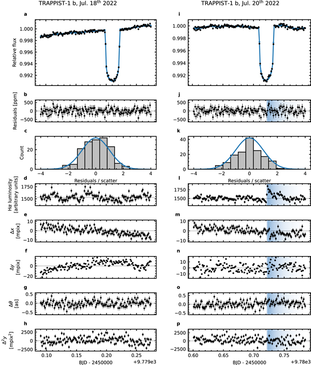
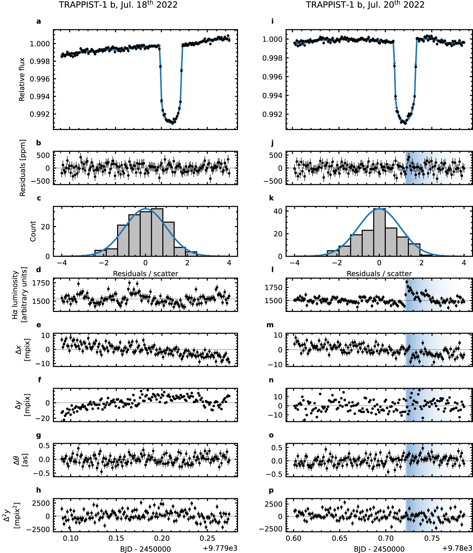
Figure 1. NIRISS/SOSS broadband light-curve fits, Hα integrated flux, and spectral trace morphology metrics. Panels (a)–(h) correspond to visit 1 and panels (i)–(p) to visit 2. All error bars are 1σ uncertainties. (a) & (i) Observed light curve (black points) and best-fit model (blue curve). (b) & (j) Light-curve residuals from the best-fit model. (c) & (k) Histogram of the light-curve residuals normalized by the scatter (bars) and a Gaussian distribution (blue curve) for comparison. (d) & (l) Time series of the integrated flux of the Hα stellar line. (e) & (m) Amplitude of the trace displacement in the spectral direction (b(t) in text). (f) & (n) Amplitude of the trace displacement in the cross-dispersion direction (c(t)). (g) & (o) Amplitude of the trace rotation (d(t)). (h) & (p) Amplitude of the second derivative of the trace profile in the cross-dispersion direction (e(t)). For visit 2, the shaded blue domain highlights the stellar flare. The jump in the broadband flux (j) and in the Hα integrated flux (l) are not linked to any anomaly in the spectral trace morphology ((m)–(p)).
Download figure:
Standard image High-resolution image4. Transit Light-curve Fitting
With the extracted spectra, we performed a global analysis of the broadband and spectroscopic transit light curves with ExoTEP (Benneke et al. 2017, 2019;Benneke 2019; see Appendix B).
On top of long-timescale flux modulations such as a slope or a curvature, the light curves from both visits exhibit correlated noise on shorter timescales (e.g., around the transit egress of visit 2; see Figure 1(i)). These temporal flux variations are correlated with the wavelength-integrated flux of the Hα stellar line (see Figure 1(l) and Appendix C), and are not correlated with any spectral trace morphological metrics we computed (e.g., trace displacement; see Figures 1(m)–(p)), which is suggestive of a stellar, not instrumental, nature of the correlated noise. We interpret the bump in the second transit as a stellar flare. Had we not detected the Hα line variability, we could have mistaken this structure in the second transit for a spot-crossing event (3.5σ detection using SPOTROD; 17 Béky et al. 2014). The Hα line is thus an important proxy for stellar flares, and its variability is more unambiguously detected when its spectral resolution is higher because the line is then less diluted, giving an edge to NIRISS/SOSS relative to NIRSpec/Prism (see also Howard et al. 2023).
Given these short-timescale correlated noise structures, we performed the broadband and spectroscopic transit light-curve analyses with five different systematics treatments, including Gaussian processes (GPs; Rasmussen & Williams 2006; Ambikasaran et al. 2015) and detrending against the integrated flux of the Hα stellar line (see Appendix B.3). All five systematics treatments resulted in statistically consistent transit spectra (Appendix B.3). The GP approach performed the best in terms of correlated noise removal, and therefore unless otherwise stated, the quantitative results presented hereafter are derived from transit spectra resulting from this treatment (Figures 2(a)–(b)).
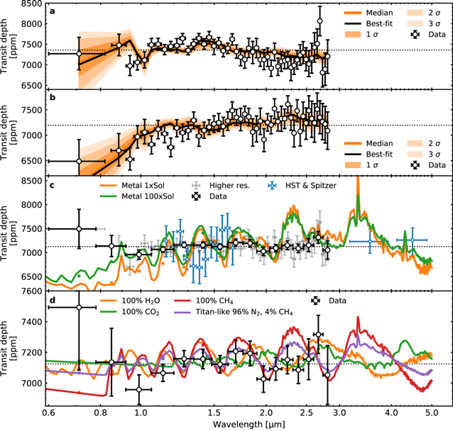
Figure 2. NIRISS/SOSS transit spectra of TRAPPIST-1 b compared to stellar-contamination and atmosphere models from the sequential analysis. Black circles are the SOSS transit spectra, either from visit 1 (a), visit 2 (b), or from both visits combined ((c)–(d)). In panels (c) and (d), the transit spectra are corrected from stellar contamination. Dashed lines are the error-weighted mean transit depths. Vertical error bars are 1σ uncertainties. Horizontal error bars represent the extent of each spectral bin. (a)–(b) Comparison between the transmission spectrum of each visit to its best-fit/median stellar-contamination model (black/orange curves) and uncertainties (shaded regions). (c) Gray, thin error bars are the SOSS transit depths at higher spectral resolution. Blue points are the Hubble Space Telescope (HST)/WFC3 and Spitzer/IRAC transit depths (de Wit et al. 2016, 2018; Zhang et al. 2018; Ducrot et al. 2020a), vertically shifted to match the median of the SOSS data. Clear, hydrogen-rich models in orange and green can be ruled out at 29 and 16σ, respectively. (d) Clear 100% CH4 (red), CO2 (green), H2O (orange), and Titan-like (purple) atmospheres cannot be rejected or confirmed.
Download figure:
Standard image High-resolution image5. Stellar-contamination and Planetary Atmosphere Fits
We investigated the contribution of stellar contamination from unocculted starspots and/or faculae (Sing et al. 2011; McCullough et al. 2014; Rackham et al. 2017, 2018, 2023) to the transmission spectra through two different fitting approaches. The first approach fits a stellar-contamination model to the transmission spectrum of each of the two visits. The best-fitting stellar-contamination model for each visit is then divided out from each transmission spectrum, and the error-weighted average of the two stellar-contamination-corrected spectra is then subjected to a planetary atmosphere retrieval—we term this approach a sequential fit of the stellar contamination and planetary atmosphere (Section 5.1). The second approach jointly fits a stellar-contamination and planetary atmosphere model to each transit spectrum—we term this a simultaneous fit of the stellar contamination and planetary atmosphere (Section 5.2).
An alternative approach to treat stellar contamination is to fit the out-of-transit stellar spectra to constrain the heterogeneity properties, and then use these constraints to correct the transmission spectrum (Wakeford et al. 2019; Zhang et al. 2018; Garcia et al. 2022; Rackham & de Wit 2023; Berardo et al. 2023). This approach has the advantage of using information from the star only to correct for stellar contamination, in contrast to the fit to the transmission spectrum, which could be biased by the signal of a planetary atmosphere, thereby possibly erasing part of the planetary contribution during the stellar-contamination correction.
However, all of these approaches use theoretical stellar spectra such as the PHOENIX ACES models (Husser et al. 2013), which struggle to reproduce the observed, out-of-transit, spectrum of TRAPPIST-1, a late-type ultracool dwarf (see Appendix D). These limitations in model fidelity impart an accuracy bottleneck in analyses of stellar impacts on transmission spectra and prevent us from determining the number of heterogeneities needed for contamination correction, resulting in error bars in the corrected transmission spectra that should actually be ∼1000–2000 ppm per native-resolution pixel (as seen in Wakeford et al. 2019; Garcia et al. 2022; Rackham & de Wit 2023; and per the work in Appendix D), whether we fit the out-of-transit stellar spectra or the transmission spectra. These limitations also imply that the inferred spot and facula parameters likely do not reflect the true state of the heterogeneities at the time of the observations. This lack of model fidelity calls for more theoretical work and/or continuous observations of the star to characterize the heterogeneities empirically (see, e.g., Rackham et al. 2023). We did not apply the method based on out-of-transit spectra because for this particular approach the mismatch of the models to the data may lead to a stellar-contamination correction that is largely inconsistent with the actual contribution of contamination to the transmission spectra.
5.1. Sequential Fit
The stellar-contamination model assumes that the visible stellar disk has two unocculted regions, a spot and a facula, for a total of three components, including the quiescent photosphere. We opted for three components as it is the simplest model that allows one component to be hotter and one colder than the quiescent photosphere. The covering fractions of the spot and facula can go to zero, hence allowing a two- and a single-component scenario. We did not compare our results with models with more components, as the reduced χ2 values were already close to 1, i.e., the three-component model already provided a reasonable fit to the observations (Section 6.1). However, we do acknowledge that the transit depth precision may be underestimated because it does not fully account for the uncertainty on the number of components. More analysis, and likely more observations, will be needed to determine the number of components that best fit the data.
We compute a weighted average of three PHOENIX ACES stellar spectra (Husser et al. 2013) at the temperatures and gravities of each component to simulate the spectrum of a heterogeneous disk. The weight of each spectrum is determined by the size of the spot and of the facula. We then compute the expected transmission spectrum assuming an atmosphere-less planet transiting this heterogeneous disk (Equation (3) from Rackham et al. 2018).
Since the two visits were approximately 1.5 days apart (Gillon et al. 2017) and adopting a stellar rotation period of 3.3 days (Luger et al. 2017), the two visits were about half a stellar rotation apart, meaning that the spot and facula properties can be different between these two visits. We thus fitted the stellar-contamination model to the transit spectrum of each visit separately, inferring the properties of the unocculted stellar heterogeneities, i.e., their temperature differences with respect to the quiescent photosphere, surface gravities, and covering fractions, with the priors listed in Table 1. We forced the sum of both covering fractions to remain smaller than 1. Following Fournier-Tondreau et al. (2023), we set the surface gravity as a free parameter as a proxy of the pressure in the heterogeneity, which may be affected by the presence of magnetic fields (Solanki 2003; Bruno et al. 2021). For simplicity, we forced both heterogeneities to have the same surface gravity in this particular fit. We also set the planet-to-star radius ratio and the photospheric temperature as free parameters to account for their uncertainties.
Table 1. Priors and Posteriors of the Stellar-contamination Parameters from the Sequential and Simultaneous Fits of the Stellar Contamination and Planetary Atmosphere
| Stellar-contamination Parameter | Priors | Posteriors | ||||
|---|---|---|---|---|---|---|
| Sequential | Simultaneous | Sequential | Simultaneous | |||
| Visits 1 & 2 | Visits 1 & 2 | Visit 1 | Visit 2 | Visit 1 | Visit 2 | |
| Spot covering fraction, fspot |

|

|

|

|

|

|
| Facula covering fraction, ffac |

|

|

|

|

|

|
| Photospheric temperature, Tphot (K) |

|

|

|

|

|

|
Stellar photosphere gravity,  (dex) (dex) | 5.0 |

| 5.0 | 5.0 |

|

|
| Spot temperature, Tspot or ΔTspot (K) |
 a
a
|
 b
b
|
 a
a
|
 a
a
|
 b
b
|
 b
b
|
| Facula temperature, Tfac or ΔTfac (K) |
 a
a
|
 b
b
|
 a
a
|
 a
a
|
 b
b
|
 b
b
|
Spot surface gravity,  (dex) (dex) |

|

|

|

|

|

|
Facula surface gravity,  (dex) (dex) |

|

|

| |||
| Planet radius Rp (R⊕) | ... |
|

|

|

|

|
Planet-to-star radius ratio, squared  (ppm) (ppm) |
| ... |

|

|

|

|
Notes. In the prior columns, T⋆,eff = 2566 K,  , and Rp,obs = 1.116 R⊕ are adopted from the literature (Agol et al. 2021), with slightly more conservative uncertainties
  and
and  , and med(Tdepth) is the median of the measured transit depths of each visit. In the posterior columns, the leftmost value is the 50th percentile of the posterior distribution. Upper and lower uncertainties are computed from the 16th, 50th, and 84th percentiles.
Download table as: ASCIITypeset image
We then divided out the median stellar-contamination model from each of the two transmission spectra and multiplied back the median squared planet-to-star radius ratio. We took an error-weighted average of the two stellar-contamination-corrected transmission spectra, yielding a stellar-contamination-corrected and combined transmission spectrum.
Before performing the planetary atmosphere retrieval, we first compared the stellar-contamination-corrected and combined transmission spectrum to a selection of SCARLET planetary atmosphere forward models (Benneke & Seager 2012, 2013; Benneke 2015, 2019; Benneke et al. 2019; Pelletier et al. 2021) of TRAPPIST-1 b. We computed the χ2 statistic between each atmospheric model and the corrected and combined spectrum, and measured how far out in the distribution tail the statistic fell, in units of the standard deviation of the χ2 distribution (Gregory 2005). This frequentist calculation provides us with rejection (or detection) confidence levels for specific planetary atmosphere scenarios, which can guide the atmospheric retrieval.
We used SCARLET to perform a planetary atmosphere retrieval on the stellar-contamination-corrected and combined transmission spectrum. Since the frequentist comparison between atmospheric forward models and the corrected and combined spectrum did not detect an atmosphere, this retrieval analysis explored the range of mean molecular masses and surface/cloud pressures that remain consistent with the data, similar to an analysis done with GJ 1214 b and GJ 436 b (Benneke & Seager 2013; Kreidberg et al. 2014; Knutson et al. 2014). We used a parameter space that efficiently samples the full range of models between hydrogen-dominated and volatile-dominated atmospheres. We adopted a mix of H2/He at solar ratio, along with molecules of higher mean molecular mass, namely H2O, CH4, CO, CO2, NH3, and N2. This is because TRAPPIST-1 planets could host a wide variety of secondary atmospheres with outgassing/volcanism and cometary delivery as their main sources (Turbet et al. 2020 and references therein), along with photochemistry shaping the composition of these atmospheres given the strong X-ray and UV radiation and flares emitted by the host star (Wheatley et al. 2017; Bourrier et al. 2017; Vida et al. 2017). Optically thick and gray clouds were also included in the model, such that the pressure parameter corresponds to the pressure either at the ground or at the top of the cloud. We parameterized the forward model to sample the pressure and H2/He abundance relative to all gases, using the two-component centered-log-ratio transform (Benneke & Seager 2013), also illustrated by the horizontal axis stretch of Figure 3.

Figure 3. Joint constraints on the H2/He abundance and the atmospheric pressure on TRAPPIST-1 b resulting from the sequential fit of the stellar contamination and planetary atmosphere. The color shading illustrates the posterior probability density, where darker colors correspond to higher probabilities. Contours indicate the 1σ, 2σ, and 3σ Bayesian credible regions. The displayed posterior probability is marginalized over the H2O, CH4, CO, CO2, NH3, and N2 abundances. Hydrogen-dominated scenarios with high-altitude clouds are at the top left corner of the plot and cloud-free, volatile-rich, high-mean-molecular-mass atmospheres are at the bottom right. Any hydrogen-rich atmospheres without high-altitude clouds, at the bottom left, are robustly ruled out. The second horizontal axis at the top shows the mean molecular mass representative for a pure H2/H2O atmosphere.
Download figure:
Standard image High-resolution image5.2. Simultaneous Fit
For the simultaneous fit of the stellar contamination and planetary atmosphere, we used POSEIDON (MacDonald & Madhusudhan 2017; MacDonald 2023) to analyze the transmission spectrum of each visit individually. We parameterized stellar contamination via a two-heterogeneity model defined by eight free parameters (Fournier-Tondreau et al. 2023; priors listed in Table 1): the spot and facula coverage fractions, temperatures, and local surface gravities, as well as the stellar photosphere temperature and surface gravity. We calculated the impact of stellar contamination by interpolating PHOENIX models (Husser et al. 2013) using the MSG package (Townsend & Lopez 2023). We fitted for the planetary atmosphere via a six-parameter model: the atmosphere radius at the 1 bar reference pressure, Rp,ref (with prior  , where Rp,obs = 1.116 R⊕; Agol et al. 2021), the atmospheric temperature, T (
 K), and the H2, H2O, and CO2 mixing ratios, Xi
(centered-log-ratio priors from 10−12 to 1 with the remainder of the atmosphere filled with N2; Lustig-Yaeger et al. 2023). We calculated each model transmission spectrum on a wavelength grid at a resolving power of R = 20,000 from 0.58 to 3.0 μm, including both the planetary atmosphere and stellar-contamination contribution.
K), and the H2, H2O, and CO2 mixing ratios, Xi
(centered-log-ratio priors from 10−12 to 1 with the remainder of the atmosphere filled with N2; Lustig-Yaeger et al. 2023). We calculated each model transmission spectrum on a wavelength grid at a resolving power of R = 20,000 from 0.58 to 3.0 μm, including both the planetary atmosphere and stellar-contamination contribution.
6. Results and Discussion
6.1. Evidence for Stellar Contamination
The transmission spectra of TRAPPIST-1 b notably differ between the two visits (Figures 2(a)–(b)), with different wavelength-dependent slopes, spanning a few hundreds of parts per million, and different absorption band-like features. These differences can be explained by stellar contamination and its variation between the two epochs.
The stellar-contamination fit of the sequential fit shows that the transmission spectrum of the first visit is explained by an unocculted spot (with no evidence for faculae), with a covering fraction of  and a temperature difference with respect to the photosphere of
  K (Figure 2(a) and Table 1). The second visit shows a preference for an unocculted facula (with no evidence for spots), causing the strong slope in the blue part of the spectrum (Figure 2(b)). The covering fraction of this facula is
  and its temperature difference is
  K. The stellar-contamination model cannot perfectly fit the observed spectra, which is explained by the mismatch between the stellar models and the observations (see Appendix D), but it can, to some extent, explain the slope blueward of 1.3 μm as well as some features near 1.4 μm, especially for the second visit.
The results from the simultaneous stellar-contamination and planetary atmosphere fit (Figure 4 and Appendix E) are consistent with the unocculted spot and faculae properties inferred from the stellar-contamination fit of the sequential fit (Table 1). The first visit is explained by unocculted spots about 200 K cooler than the stellar photosphere, while the second visit requires unocculted faculae about 160 K hotter than the photosphere (Figures 4(c)–(d)). The stellar-contamination model is moderately to strongly preferred over a flat spectrum model, with log Bayes factors of 5.3 and 2.9 for the first and second visits, respectively, following Table 1 from Trotta (2008). Comparing the transmission spectra from the two visits to a stellar-contamination-only model and a joint stellar-contamination and planet atmosphere model (Figures 4(a)–(b)) shows that the observations can be described by stellar contamination alone; there is no significant improvement from adding an atmosphere. The χ2 from the fits are as follows: for visit 1, χ2 = 44.0 (with 41 degrees of freedom) for a retrieval with only stellar contamination and 43.5 (with 37 degrees of freedom) for stellar contamination and a planetary atmosphere. For visit 2, χ2 = 30.6 and 29.6 for the same models.
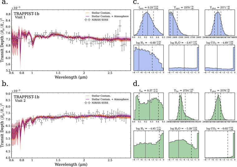
Figure 4. Atmospheric and stellar properties from the transmission spectra of TRAPPIST-1 b from the simultaneous stellar-contamination and planetary atmosphere fit. (a)–(b) Retrieved model spectrum of TRAPPIST-1 b from two retrievals: a stellar-contamination model with unocculted spots and faculae (orange) and a joint stellar-contamination and planetary atmosphere model (purple), for visits 1 and 2. The median retrieved model (solid lines) and the corresponding 1σ and 2σ confidence intervals (dark and light contours, respectively) are compared to the observed TRAPPIST-1 b spectrum (black points). Error bars are 1σ uncertainties. (c)–(d) Corresponding posterior probability distributions from the joint stellar-contamination and planetary atmosphere retrieval for visits 1 and 2. The TRAPPIST-1 b spectra are well fitted by the stellar-contamination model ( = 1.07 and 0.75 for the best-fitting model spectra to visits 1 and 2, respectively), with no fit improvement from adding a thick planetary atmosphere. However, the CO2 and H2O posteriors indicate that a high-mean-molecular-mass atmosphere remains consistent with the TRAPPIST-1 b observations.
Download figure:
Standard image High-resolution imageThe inferred stellar heterogeneity parameters and atmospheric constraints from the simultaneous fit are generally similar to those inferred from the sequential fit (Section 6.2), likely due to the lack of features from the planetary atmosphere. These two analyses of the NIRISS/SOSS observations strongly support previous evidence that stellar contamination is a critical consideration when interpreting any transmission spectrum of planets transiting active stars (e.g., Moran et al. 2023), in particular TRAPPIST-1 planets (Zhang et al. 2018; Wakeford et al. 2019; Ducrot et al. 2020; Garcia et al. 2022). It is intriguing though that the amplitude of the TLS effect is over an order of magnitude larger in the two TRAPPIST-1 b spectra (∼750–1000 ppm peak to peak) than in the TRAPPIST-1 g spectra obtained with NIRSpec/Prism over two visits (B. Benneke et al. 2023, in preparation), also part of the JWST TRAPPIST-1 atmospheric reconnaissance program. This may indicate that the amplitude of the TLS effect varies strongly with epoch and/or transit impact parameter (b ∼ 0.1 and b ∼ 0.4 for TRAPPIST-1 b and g, respectively; Agol et al. 2021), but this remains speculative given the small number of observations. All this underscores the need for more observations to quantify better the impact of stellar contamination at any given epoch and geometrical configuration.
6.2. Constraints on the Planetary Atmosphere
The median error bar of the stellar-contamination-corrected and combined transmission spectrum at R ∼ 15 is 89 ppm, not accounting for the ∼1800 ppm per-pixel model-driven uncertainty associated with the lack of stellar model fidelity (see Appendix D). Signatures of a cloud-free atmosphere on TRAPPIST-1 b could have amplitudes of 100–200 ppm, depending on the exact atmospheric conditions (Lincowski et al. 2018). The precision achieved with two NIRISS/SOSS transits is thus insufficient to detect or reject such atmospheres confidently yet, but it shows that this objective could be within reach with a reasonable number of visits considering the expected lifetime of JWST and its instrument.
The frequentist comparison between atmospheric forward models and the stellar-contamination-corrected and combined transmission spectrum rejects cloud-free, hydrogen-rich atmospheres at 1× and 100× solar metallicity at 29 and 16σ, respectively, further confirming previous analyses of HST observations (de Wit et al. 2016). We also compared the transmission spectrum to a limited set of cloud-free secondary atmospheres, namely pure CH4, H2O, and CO2 models, as well as a clear Titan-like scenario (Figure 2(d)), but none of these scenarios can be confidently confirmed or rejected at present (0.82, 0.48, 0.84, and 0.44σ, respectively). We conclude that the current NIRISS transmission spectrum (two visits), after stellar-contamination correction, does not show any signatures of an atmosphere.
The sequential fit of stellar contamination and planetary atmosphere finds that the TLS-corrected and combined transmission spectrum is only consistent at 3σ with a particular range of atmospheres (Figure 3), from clear atmospheres with a mean molecular mass greater than approximately 9 amu to low-mean-molecular-mass atmospheres with cloud surface pressures less than 0.1 bar. However, if TRAPPIST-1 b has retained a primordial atmosphere, cloud formation could be unlikely given the amount of radiation the planet receives (Morley et al. 2015; de Wit et al. 2016). Clouds are also unlikely, at least on the dayside of TRAPPIST-1 b, given the near-zero Bond albedo inferred from the JWST/MIRI secondary eclipse observations (Greene et al. 2023). These Bayesian results are consistent with the frequentist rejection of the clear hydrogen-rich forward models.
The simultaneous fit of stellar contamination and planetary atmosphere finds a 3σ upper limit on the H2 abundance of 52% from the first visit (Figure 4(c) and Appendix E), consistent with the results from the sequential fit. The second visit alone is inconclusive on the H2 abundance, as the faculae-dominated spectrum yields a bimodal posterior distribution, allowing an unphysical atmosphere with 100% H2 and no trace volatiles (Figure 4(d) and Appendix E). The peaks in the posteriors for H2O and CO2 are manifestations of the uninformative centered-log-ratio prior that treats all the gases equally (i.e., if there is an atmosphere with a high mean molecular mass, either or both H2O and CO2 could be the background gas). The results from this simultaneous retrieval of the planetary atmosphere and stellar contamination remain consistent with a clear, high-mean-molecular-mass atmosphere dominated by N2, H2O, and/or CO2 (see the H2O and CO2 histogram peaks in Figures 4(c)–(d)).
In addition to being consistent with pre-JWST observations, the conclusions from both the sequential and simultaneous fits of stellar contamination and planetary atmosphere are consistent with the conclusions from the JWST/MIRI secondary eclipse observations (Greene et al. 2023; Ih et al. 2023) in that the transits reveal no evidence for an atmosphere. Both the transit and secondary eclipse observations agree that TRAPPIST-1 b does not have a thick atmosphere, at least not one with a low mean molecular mass based on the transit observations. The MIRI observations provide additional constraints by rejecting certain atmospheres containing CO2, as well as atmospheres containing no CO2 for certain pressures and compositions (right panel of Figure 2 from Ih et al. 2023), further ruling out regions of the parameter space allowed by the transmission data. In this sense, the transmission spectra are less constraining in terms of atmospheric characterization for TRAPPIST-1 b, but they partially confirm the emission data and, more importantly, they bring insight into the stellar-contamination aspect of transmission spectroscopy, which is currently the preferred technique to probe the potential atmospheres of the outer, cooler TRAPPIST-1 planets.
Being closest to the host star, TRAPPIST-1 b is the planet in this system most likely to have lost its atmosphere through atmospheric escape processes. Because of the highly irradiated environment that TRAPPIST-1 b is subjected to, the potential absence of an atmosphere on TRAPPIST-1 b would not necessarily forbid atmospheres on the other planets in the system, especially the outer planets (Krissansen-Totton 2023). Moreover, the nondetection of an atmosphere on TRAPPIST-1 b can provide insight into the evolutionary history of the system. Results from this work and from the eclipse observations (Greene et al. 2023; Ih et al. 2023) should thus not discourage anyone from monitoring transits of the TRAPPIST-1 planets to search for atmospheric signatures.
7. Conclusion
We presented the first transmission spectra of the TRAPPIST-1 b planet with NIRISS/SOSS. Stellar contamination, whose manifestation differs from one visit to the other, dominates the transmission spectra at the level of several hundreds of parts per million and must be properly disentangled from planetary signals. Accounting for stellar contamination, our analyses confidently reject clear H2-rich atmospheres for TRAPPIST-1 b. However, the current SOSS observations cannot confirm whether TRAPPIST-1 b is a bare rock or if it has a thin and/or high-mean-molecular-mass atmosphere, although the latter scenario has been rejected for certain compositions by secondary eclipse observations with JWST/MIRI (Greene et al. 2023; Ih et al. 2023). As TRAPPIST-1 b is the planet in the system most likely to have lost its atmosphere (Krissansen-Totton 2023), a lack of atmosphere would not suggest that the outer planets are bare rocks and thus should not discourage future observations of the TRAPPIST-1 system. Assessing the presence of an atmosphere on the habitable-zone and outer TRAPPIST-1 planets is currently only possible with transmission spectroscopy. Given the lack of stellar model fidelity, additional theoretical work (e.g., Witzke et al. 2022; Rackham et al. 2023) and/or observations of the host star (e.g., Berardo et al. 2023) are necessary to provide better constraints on the contribution of stellar contamination to future transmission spectra.
Acknowledgments
This work is based on observations made with the NASA/ESA/CSA James Webb Space Telescope. The data were obtained from the Mikulski Archive for Space Telescopes at the Space Telescope Science Institute, which is operated by the Association of Universities for Research in Astronomy, Inc., under NASA contract NAS 5-03127 for JWST. These observations are associated with program #2589. This research has made use of the VizieR catalog access tool, CDS, Strasbourg, France. Specifically, VizieR catalog J/A + A/640/A112 (Ducrot et al. 2020b) was used to produce Figure 2(c). The original description of the VizieR service was published in 2000, A&AS 143, 23. O.L. acknowledges financial support from the Fonds de recherche du Québec – Nature et technologies (FRQNT), and funding from the Trottier Family Foundation in their support of iREx. B.B. acknowledges financial support from the Natural Sciences and Engineering Research Council (NSERC) of Canada and the FRQNT. R.D. acknowledges financial support from the NSERC and the Canadian Space Agency through grants number 22JWG01-3 and 22EXPJWST. R.J.M. acknowledges support for this work provided by NASA through the NASA Hubble Fellowship grant HST-HF2-51513.001 awarded by the Space Telescope Science Institute, which is operated by the Association of Universities for Research in Astronomy, Inc., for NASA, under contract NAS 5-26555. C.P. acknowledges financial support from the FRQNT, the Technologies for Exo-Planetary Science (TEPS) Trainee Program and the NSERC Vanier Scholarship. A.L'H. and M.F.-T. acknowledge financial support from the FRQNT. B.V.R. thanks the Heising-Simons Foundation for support. This material is based upon work supported by the National Aeronautics and Space Administration under Agreement No. 80NSSC21K0593 for the program "Alien Earths." The results reported herein benefited from collaborations and/or information exchange within NASA's Nexus for Exoplanet System Science (NExSS) research coordination network sponsored by NASA's Science Mission Directorate. L.D. acknowledges support from the Banting Postdoctoral Fellowship program, administered by the Government of Canada and the L'Oréal-UNESCO For Women in Science program. The authors wish to thank Kevin Volk for sharing the reference file required to flux calibrate the SOSS spectra of TRAPPIST-1.
Facility: JWST(NIRISS) - James Webb Space Telescope.
Software: supreme-SPOON 18 (Feinstein et al. 2022; Radica et al. 2022, 2023), ATOCA 19 (Darveau-Bernier et al. 2022), NAMELESS (Feinstein et al. 2022; Coulombe et al. 2023), jwst, 20 emcee 21 (Foreman-Mackey et al. 2013), corner 22 (Foreman-Mackey 2016), batman 23 (Kreidberg 2015), POSEIDON 24 (MacDonald & Madhusudhan 2017; MacDonald 2023), PHOENIX (Husser et al. 2013), SPHINX (Iyer et al. 2023; Iyer 2023), MSG 25 (Townsend & Lopez 2023), PyMultiNest 26 (Feroz et al. 2009; Buchner et al. 2014), astropy 27 (The Astropy Collaboration et al. 2013, 2018), numpy 28 (Harris et al. 2020), matplotlib 29 (Hunter 2007), and scipy 30 (Virtanen et al. 2020).
Appendix A: Data Reduction
A.1. supreme-SPOON
The supreme-SPOON pipeline has already been presented in detail in Radica et al. (2023; see also Feinstein et al. 2022; Coulombe et al. 2023), and the steps we follow here closely mirror those other analyses. We process the data of both visits through the standard supreme-SPOON stage 1, which includes a group-level correction of 1/f noise, and stage 2. During background correction, we found that the SOSS SUBSTRIP256 background model provided by STScI could not completely remove the pick-off mirror jump in the zodiacal background near spectral pixel 700 in Figure 5(b). We therefore constructed a new background model from a high signal-to-noise ratio (S/N) stacked image of each TRAPPIST-1 time series. We first masked all traces (target and field contaminants) and bad pixels. Then, assuming each column sees a constant background level, we adopted the 10th percentile value of each column and low pass filtered these values to produce a smoothed background. We performed these steps to build the background model with the deep stack rotated such that the background discontinuity at x ≈ 700 was perfectly vertical. The model was then reprojected in 2D, derotated, and subtracted from the time series. The 1D spectral extraction was performed with a 25 pixel wide box aperture. Dilution introduced due to the overlap of the first and second spectral orders on the detector is predicted to be negligible for relative flux measurements (e.g., transmission spectra; Darveau-Bernier et al. 2022; Radica et al. 2022); we estimate that the amount of dilution introduced by the order overlap would be less than 5 ppm throughout the 0.6–2.8 μm wavelength range (following Equation (5) from Darveau-Bernier et al. 2022), significantly smaller than the transit depth precision.

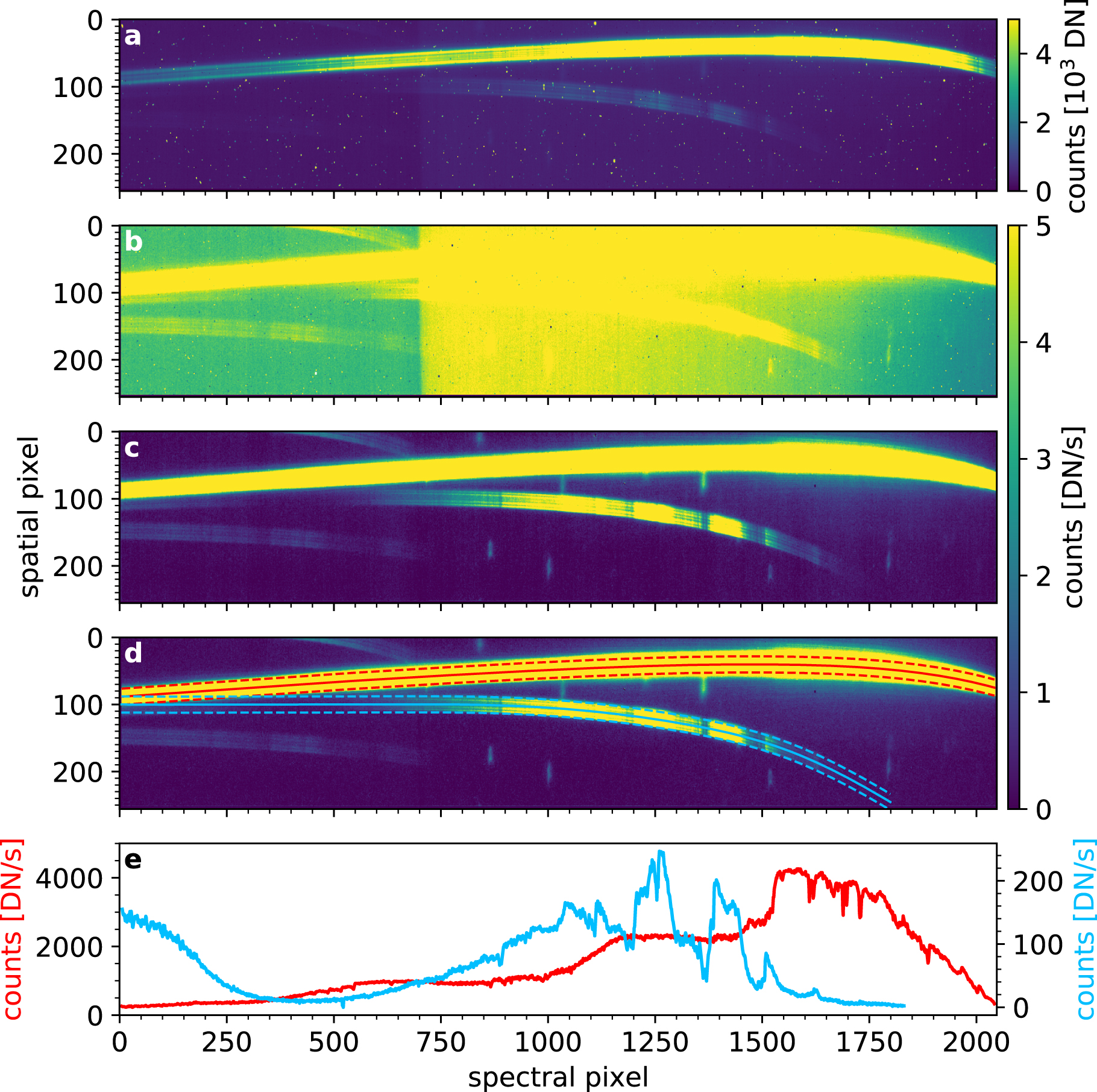
Figure 5. Reduction and spectral extraction of two SOSS spectral orders with the NAMELESS pipeline. (a) Last group of the tenth integration of visit 1, after superbias subtraction and nonlinearity correction. (b) Detector image of the tenth integration after ramp fitting of the 18 groups comprising each integration. (c) Frame after bad pixel and outlier correction, as well as background subtraction. (d) Frame after correction of the 1/f noise. The center (full line) and edges (dashed lines) of the fixed aperture boxes used to extract the first (red) and second (blue) spectral orders are shown. (e) Extracted spectra of the first (red) and second (blue) spectral orders. The sharp rise in the spectrum of the second order when going to lower spectral pixels is caused by the overlap with the first order.
Download figure:
Standard image High-resolution imageA.2. NAMELESS
We also reduced the data with the NAMELESS pipeline (Feinstein et al. 2022; Coulombe et al. 2023; Radica et al. 2023; Figure 5), which first runs all the steps of the jwst pipeline stage 1 except for dark current subtraction, as it leaves residual 1/f noise. A parallel reduction was also performed with the dark current subtraction, but it had virtually no effect on the transmission spectrum. We then went through the assign_wcs, srctype, and flat_field steps of the jwst pipeline stage 2 before performing custom routines for the correction of bad pixels, background, as well as 1/f noise (Coulombe et al. 2023).
As with the supreme-SPOON pipeline, we found that the 2D background model from STScI could not reproduce the observed background jump near spectral pixel 700. To address this issue and to avoid introducing dilution through background correction, we split the background model into two separate sections along the line tracing the jump in background flux and fitted their amplitude separately. The background model made from the two distinct sections was then subtracted from all integrations. Spectral extraction of the first and second spectral orders was performed with a 24 pixel wide box aperture.
A.3. SOSSISSE
As a third reduction pipeline, we used the SOSS-Inspired SpectroScopic Extraction (SOSSISSE) tool. The SOSSISSE tool uses rateints files, i.e., the post–ramp-fitting time series of 2D images of the trace, to express any given trace image in the time series as the linear combination of a reference trace and its spatial derivatives. This approach assumes that the trace will only suffer achromatic transforms and provides a residual map from which spectroscopic information is then retrieved. Small signals from planetary transits are thus encoded into residual maps that have a much smaller dynamic range than the input data set, such that low-amplitude effects (e.g., 1/f noise) are more readily handled.
The SOSSISSE tool first constructs a model that consists of (1) a high-S/N, normalized, out-of-transit, median trace, Mi,j , where i and j are the indices of the pixels in the x- (dispersion) and y- (cross-dispersion) directions, respectively, and (2) time-dependent morphological changes in the trace. These morphological changes are represented by spatial derivatives of Mi,j : shifts in the x- and y-directions (∂M/∂x and ∂M/∂y), a trace rotation (∂M/∂θ), and changes in the contrast of the point-spread function (PSF) structures expressed as the second derivative along the y-direction (∂2 M/∂y2). The model can be written as
where Fi,j (t) is the model trace flux at time t on pixel (i, j), and a, b, c, d, and e are time-dependent scalars (Figures 1(e)–(h) and (m)–(p)), fitted in a least-squares fashion to each 2D trace image. Scalars b, c, d, and e can be interpreted as the amplitudes of their respective derivatives (e.g., b(t) can be seen as "dx," the amplitude of the trace displacement in the x-direction).
These morphological changes in the trace should be accounted for to measure the photometric signal accurately, and the SOSSISSE tool includes them as part of the photometric measurement instead of attempting to remove them through detrending in a subsequent step. Indeed, the fitted amplitude a(t) of the high-S/N trace consistently accounts for these morphological changes in the trace, ensuring that the photometric measurements are consistent across the entire time series. We also found that e(t) is particularly effective at detecting telescope tilt events (Rigby et al. 2023; Doyon et al. 2023). These events can affect the shape of the trace, but may only slightly shift its overall position. Including this term in the model accurately captures the impact of any potential tilt events on the data.
Once an optimal trace model has been found for each 2D image of the time series, SOSSISSE subtracts this best-fit trace model from each image, leaving only chromatic temporal variations, or "residuals." SOSSISSE then collapses each 2D residual image into a 1D spectrum by performing a least-squares adjustment of the model trace F at spectral pixel (i, j) onto the residual. The underlying assumption is that residuals resulting from spectroscopic features will have the same morphology as the underlying trace. This least-squares fitting is performed with the propagation of the uncertainty from the rateints files. We also account for the probability that the per-pixel residuals are either consistent with their uncertainties or with a cosmic-ray event by giving to each pixel a weight corresponding to 1 minus its likelihood of being affected by a cosmic ray. The time series a(t), which can be interpreted as the broadband light curve, is finally added back to each spectral channel, yielding a spectral time series that can be used to perform the transit light-curve fit (Section 4).
A.4. Consistency Across Reduction Pipelines
Similar structures are present across the spectral time series of the three pipelines. For example, the temporal slope in visit 1 and the same correlated noise pattern associated with stellar activity near the transit egress in visit 2 are present in all three reductions. There are some differences between reductions, typically localized in time and wavelength, but these are expected given the differences between the pipelines.
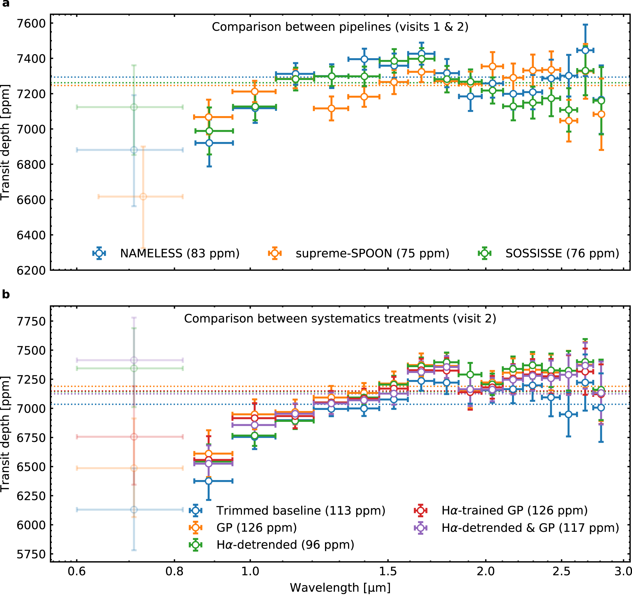
We fitted the broadband and spectroscopic light curves of all three reductions to compare the resulting transmission spectra (Figure 6(a)). Although the transit depths are generally consistent within their uncertainties, there are differences at the 100–200 ppm level in some wavelength bins. Differences of this order of magnitude between reductions have already been reported in JWST data (Feinstein et al. 2022; Coulombe et al. 2023; Rustamkulov et al. 2022; Radica et al. 2023), but these become more problematic for Earth-sized planets like TRAPPIST-1 b, whose expected atmospheric signatures have amplitudes of 100–200 ppm (Lincowski et al. 2018) at most.

Figure 6. Comparison between reductions and systematics treatments. (a) Comparison between the (combined) transmission spectra resulting from the three reduction pipelines. Solid and semitransparent points are from spectral orders 1 and 2, respectively. Horizontal dashed lines show the error-weighted average transit depths. (b) Comparison between the transit spectra of visit 2 resulting from the five different systematics treatments. In both panels, the number in parentheses in the legends is the median error bar across each spectrum. All vertical error bars are 1σ uncertainties. All horizontal error bars represent the extent of each spectral bin.
Download figure:
Standard image High-resolution imageTo assess the impact of the differences between reductions, we ran the simultaneous fit of the stellar contamination and planetary atmosphere (Section 5.2) on all three sets of TRAPPIST-1 b transmission spectra resulting from the three pipelines, generally finding consistent conclusions. Regardless of the reduction, we see evidence of stellar contamination and cloud-free, hydrogen- and helium-rich models can be ruled out at high confidence. Secondary atmospheres, especially those with a low surface pressure, and/or clouds cannot be confidently rejected from these SOSS observations. Since the conclusions remain the same across all three reductions, we consider that our reductions are reliable for the purpose of this work.
Appendix B: Transit Light-curve Fitting
B.1. Light-curve Preparation
We started the transit light-curve fit with a set of approximately 2048 light curves, with each light curve corresponding to a spectral channel. For spectral order 1, we produced the broadband light curve by binning all light curves into a single bin, whereas the spectroscopic light curves were generated by binning the light curves down to 50 bins, equally spaced in wavelength. For spectral order 2, we first removed all light curves at wavelengths above 0.82 μm, as this spectral domain is already covered by spectral order 1 (Albert et al. 2023) and removing these redder wavelengths also prevents contamination from order 1. Given the lower S/N and the fewer native-resolution channels in order 2, we only performed a broadband light-curve fit for this order. We then normalized each light curve by its median and performed 10 iterations of 3.5σ clipping to remove outliers in flux.
B.2. Broadband and Spectroscopic Light-curve Fitting
We first fitted the broadband light curves from the two visits independently with ExoTEP (Benneke et al. 2017, 2019; Benneke 2019; Figures 1(a)–(c) and (i)–(k)), which fits a batman transit model (Kreidberg 2015) and a systematics model to the light curve, along with a photometric noise parameter, using the emcee implementation (Foreman-Mackey et al. 2013) of the Markov Chain Monte Carlo method, with the priors listed in Table 2. We applied a Gaussian prior on the impact parameter based on the value and uncertainty from Agol et al. (2021) given the low temporal resolution during the transit ingress and egress. For the GP length scale (Appendix B.3), we applied a lower bound corresponding to about five integrations to prevent overfitting, and an upper bound of 2.4 hr, approximately half the duration of the observation, to prevent degeneracies with the parameters of the linear function (Appendix B.3). These independent fits of the two broadband light curves provided a first estimate of the global transit parameters (a/R⋆, b), transit ephemeris (Tmid), and transit depths in the SOSS bandpass. We then fitted the two broadband light curves simultaneously (posteriors listed in Table 2), allowing each visit to have different systematics and photometric noise parameters, initializing all parameters at their best-fit values from the individual fit to ease convergence.
Table 2. Priors and Posteriors of the Joint Broadband Light-curve Fit of the Two Visits
| White Light Curve | ||
|---|---|---|
| Parameter | Priors | Posteriors |
| Orbital period, Porb (days) | 1.51087081 | 1.51087081 |
| Midtransit time, visit 1, Tmid,1 (BJD) |

|
|
| Midtransit time, visit 2, Tmid,2 (BJD) | Tmid,1 + 1.51087081 | Tmid,1 + 1.51087081 |
| Planet-to-star radius ratio, (Rp /Rs ) | ... |

|
Planet-to-star radius ratio squared,  (ppm) (ppm) |

|

|
| Impact parameter, b |

|

|
| Quadratic LD coeff. 1, q1 |

|

|
| Quadratic LD coeff. 2, q2 |

|

|
| Eccentricity, e | 0 | 0 |
| Argument of periapsis, ω (deg) | 90 | 90 |
| Semimajor axis, a/R⋆ |

|

|
| White noise, visit 1, s1 (ppm) |

|

|
| White noise, visit 2, s2 (ppm) |

|

|
GP amplitude, visit 1, 
|

|

|
GP amplitude, visit 2, 
|

|

|
GP length scale, visit 1, 
|

|

|
GP length scale, visit 2, 
|

|

|
| Spectroscopic Light Curves | ||
|---|---|---|
| Parameters | Priors | |
| Orbital period, Porb (days) | 1.51087081 | |
| Midtransit time, Tmid (BJD) | WLC best fit | |
Planet-to-star radius ratio squared,  (ppm) (ppm) |

| |
| Impact parameter, b | WLC best fit | |
| Quadratic LD coeff. 1, q1 |

| |
| Quadratic LD coeff. 2, q2 |

| |
| Eccentricity, e | 0 | |
| Argument of periapsis, ω (deg) | 90 | |
| Semimajor axis, a/R⋆ | WLC best fit | |
| White noise (ppm) |

| |
GP amplitude, 
|

| |
GP length scale, 
|

| |
Note. For the posteriors, the leftmost value is the 50th percentile of the posterior distribution, and upper and lower uncertainties are computed from the 16th, 50th, and 84th percentiles. Posteriors are not listed for the spectroscopic light curves as they are different for each spectral bin.
We fitted the spectroscopic light curves of the two transits independently, with a transit and systematics model as well as a photometric noise parameter for each wavelength bin (Figure 7), with the priors listed in Table 2. We parameterized the quadratic limb darkening parameters following Kipping (2013). The transmission spectrum for each visit (Figures 2(a)–(b)) is given by the best-fit spectroscopic Rp/R⋆ values squared.
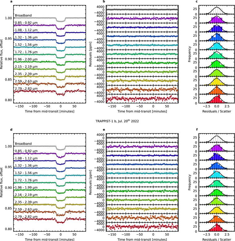
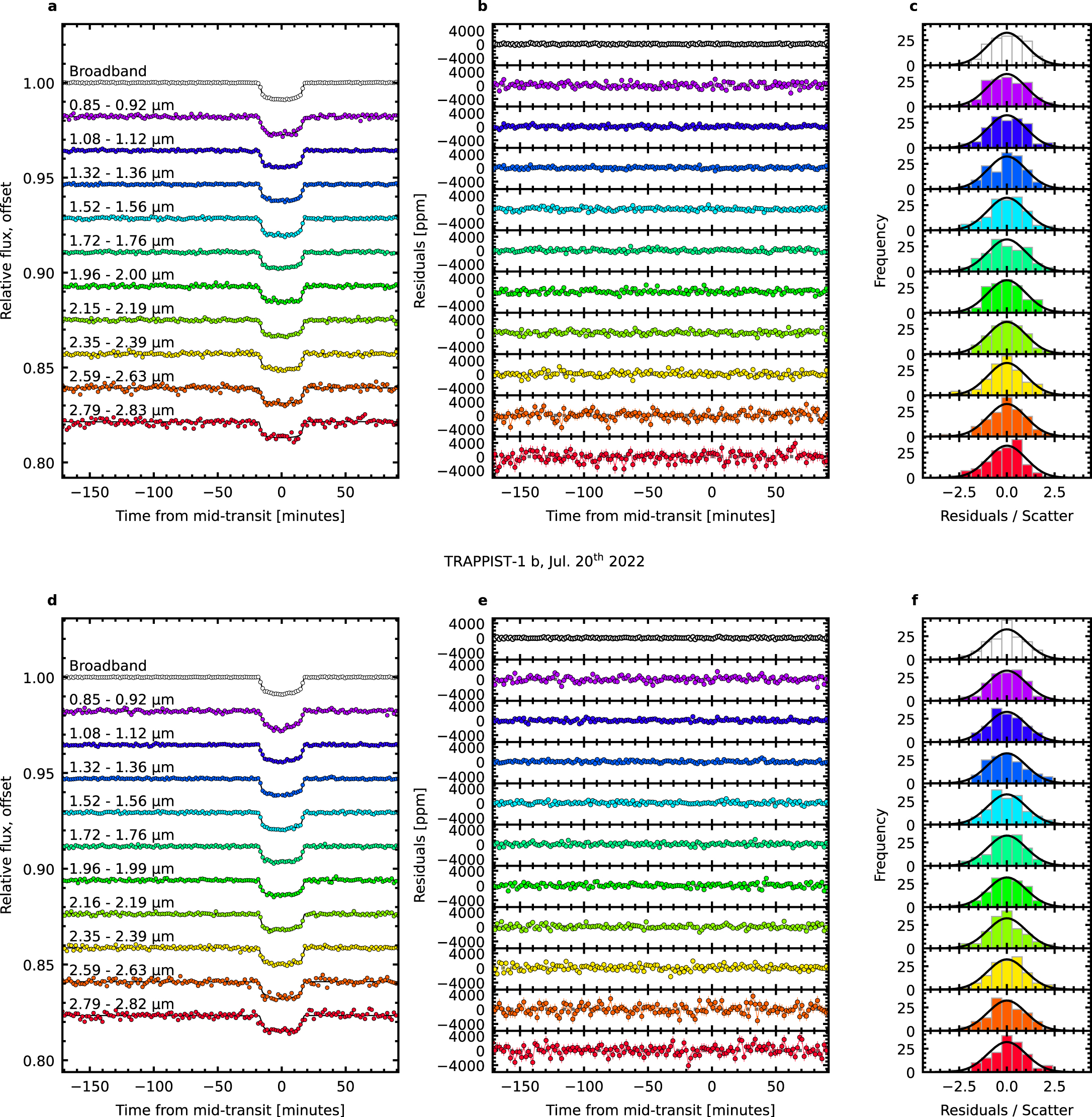
Figure 7. NIRISS/SOSS broadband (white) and spectrophotometric (colored) transit light curves. Panels (a)–(c) correspond to visit 1 and (d)–(f) to visit 2. All error bars are 1σ uncertainties. (a) and (d) Light curves. (b) and (e) Light-curve residuals from the best-fit model. (c) and (f) Distribution of the light-curve residuals, with a Gaussian distribution overplotted for comparison.
Download figure:
Standard image High-resolution imageB.3. Systematics Treatment
The broadband light curve of the second visit (Figure 1(i)) betrays the presence of 3–15 minute long correlated noise structures produced by stellar activity (Section 4). This correlated noise is most easily seen as flux variations before and after the transit egress of the second visit, but more subtle modulations are also present elsewhere in both visits. To mitigate the impact of this correlated noise on the measured transit depths, we tested two different systematics treatments for both transits, and three additional treatments for the second visit, specifically to leverage the apparent correlation between the Hα integrated flux and the flux in other wavelength bins. We tested each of these five systematics treatments in parallel during the transit light-curve fitting (Appendix B.2). In all five systematics treatments, we used a linear function as the basic systematics model S(t), such that the most basic flux model is written as
where f0 is the baseline flux, T(t, θ) is the transit model, v and c are the slope and normalization constant of the linear function, respectively, and t0 is the time at the start of the visit.
The first systematics treatment consisted of trimming the baseline and masking temporally correlated points such that the most obviously correlated noise patterns would not affect the fit. For visit 1, we removed 2 hr and 0.6 hr from the start and the end of the visit, respectively. For visit 2, we masked six in-transit and 12 posttransit points, all of which seemed correlated in time and with Hα. We also removed 2 hr from the start, but did not remove any additional parts from the end, since 12 points were already masked, such that trimming would have left very little posttransit baseline.
The second systematics treatment consisted in using a GP (Rasmussen & Williams 2006). We used a squared-exponential kernel to define the covariance matrix of the likelihood function using the george Python package (Ambikasaran et al. 2015), keeping the white photometric noise parameter on the diagonal of the covariance matrix, added in quadrature to the kernel function. This added two free hyperparameters to the fit of each light curve: the amplitude aGP and timescale λGP of the GP.
The subsequent systematics treatments were only applied to the second visit as they all involved the Hα luminosity, which was most obviously correlated with the flux at other wavelengths for this visit. The third systematics treatment consisted of detrending the light curves against the Hα integrated flux, that is

where w is a free parameter for each light curve, FHα (t) is the Hα luminosity time series, and FHα,0 is the Hα luminosity at the start of the visit.
In the fourth systematics treatment, we first trained a squared-exponential kernel GP on the Hα luminosity time series, yielding a Gaussian-like posterior distribution function (PDF) for both aGP and λGP. We used the mean and standard deviation of the PDF of λGP to define a Gaussian prior applied to λGP as we fitted the broadband and spectroscopic light curves with a squared-exponential kernel GP.
The fifth systematics treatment was a combination of the second and third treatments, that is, detrending against the Hα luminosity and using a (untrained) squared-exponential kernel GP.
Transit depths are consistent within their uncertainties across all systematics treatments (Figure 6(b)). This shows that the GP does not bias the measured Rp/Rs, at least not in a way that is different from simply masking parts of the light curves or simply detrending against the Hα luminosity. The median error bars, in parentheses in the legend, are larger for the trimmed baseline treatment and any treatment involving a GP. The larger error bars for the trimmed baseline treatment is simply explained by the reduced amount of data, especially in visit 2 where in-transit points were masked. We explain the larger error bars in the GP treatments by the fact that the GP hyperparameters may be correlated with the transit depths, which inflates their error bars. However, a smaller median error bar on the transit depths does not necessarily mean a better fit to the light curves. A visual inspection of the light-curve residuals from the best-fit model of each wavelength bin for each systematics treatment indicated that the uninformed GP (treatment 2) provided a better fit, that is, it yielded residuals with the least correlated noise. This is expected given its more flexible nature compared to detrending against the fixed Hα time series. This is why we selected treatment two as our reference.
Appendix C: Stellar Variability
The extracted light curves of the two visits showed numerous indicators of stellar variability. The average out-of-transit linear slope of the broadband light curve of visit 1 was 8.21 ± 0.24 ppm minute−1, within the range of values inferred from the K2 light curve (±10 ppm minute−1, computed from Luger et al. 2017). For visit 2, the out-of-transit baseline had a curvature that could not be properly described by a linear function, consistent with an inflection point in the K2 light curve. Since the two visits were approximately 1.5 days apart (Gillon et al. 2017), and assuming the stellar flux is modulated with a period of 3.3 days (Luger et al. 2017), it would be possible for the first visit to be in a phase of increasing stellar flux and the second, at an inflection point. During commissioning, two other stars showed different slope values in their light curves (Doyon et al. 2023), suggesting that the flux variations seen in the TRAPPIST-1 data are astrophysical, not instrumental.
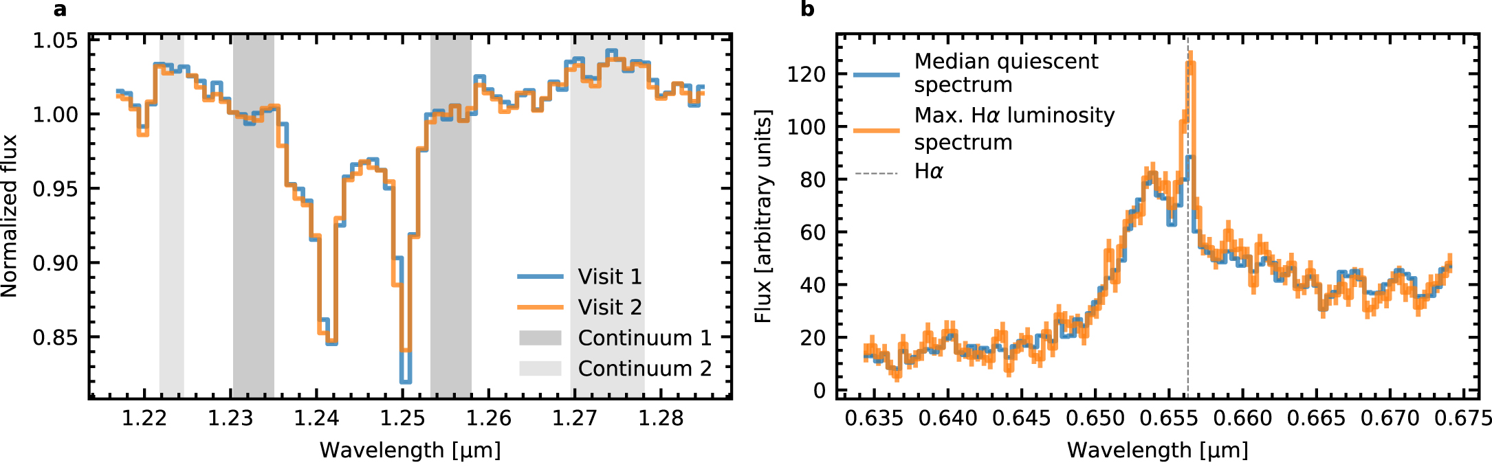
The temperature-sensitive K i doublet at 1.24–1.25 μm (Geballe et al. 2001; Fuhrmeister et al. 2022) was detected in both visits (Figure 8(a)). The average equivalent width (EW) of the reddest of the two lines is 4.134 ± 0.003 and 4.034 ± 0.003 Å for visits 1 and 2, respectively, adopting the dark shaded region in Figure 8(a) as the continuum. Using the light shaded region in Figure 8(a) as the continuum instead, we measured 5.510 ± 0.003 and 5.338 ± 0.003 Å. We used PHOENIX ACES models (Husser et al. 2013) to convert this temporal variation of the K i EW into a variation in effective temperature to infer that the average photosphere of visit 1 was, depending on our definition of the continuum, 15.3 ± 0.6 or 19.7 ± 0.4 K cooler than visit 2. We adopt 18 ± 3 K as the average photosphere temperature variation between visits 1 and 2, roughly consistent with the photometric peak-to-peak variability of about 2% of the K2 light curve (Luger et al. 2017).

Figure 8. Signatures of stellar variability and activity between and within the two visits. (a) Median extracted spectrum of visits 1 (blue) and 2 (orange), zoomed in on the 1.24–1.25 μm K i doublet. Uncertainties are smaller than the line width. Shaded regions show the two different definitions of the continuum adopted to compute the EW of the reddest of the two lines of the doublet. (b) Median quiescent (out-of-flare) stellar spectrum of visit 2 (blue) and stellar spectrum at maximum Hα luminosity (orange), i.e., at the peak of the flare in visit 2. Error bars are 1σ uncertainties.
Download figure:
Standard image High-resolution imageThe Hα stellar line was also detected and showed significant variability within and between visits (Figures 1(d) and (l) and 8(b)). Continuum flux was correlated with Hα as evidenced by the small flare event in the broadband light curve of visit 2, near egress (compare Figures 1(j) and (l)). Such continuum variation is a clear source of systematic uncertainty for transit depth measurements, hence the five systematics treatments tested (Appendix B.3). More TRAPPIST-1 observations may be used to derive an empirical calibration between Hα and the continuum flux to correct light curves from stellar activity signals, which will likely be very common in this system.
Appendix D: Stellar Spectrum
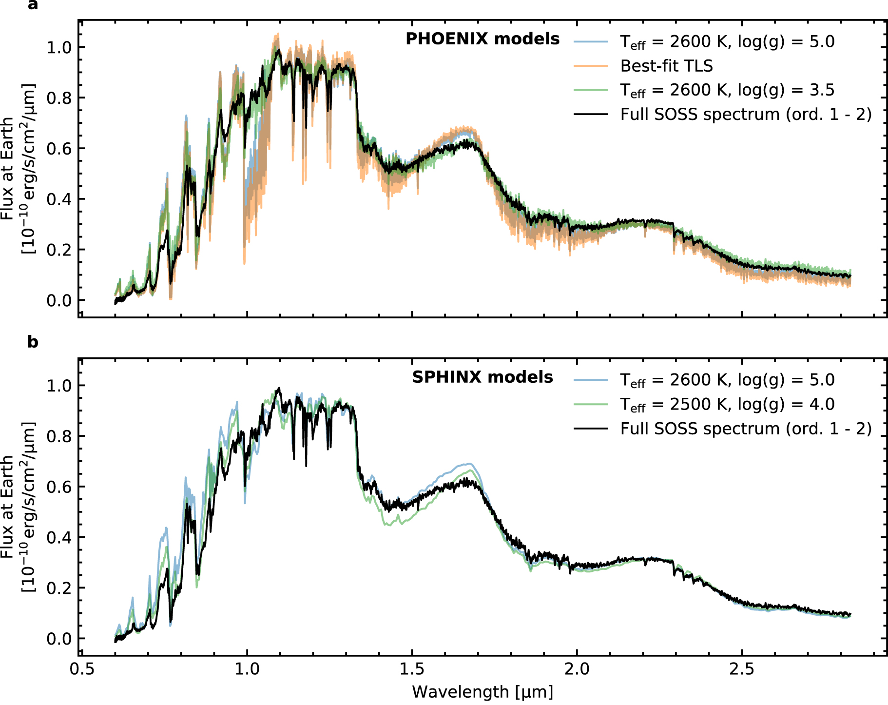
To expand on the discrepancies between the theoretical stellar spectra and observations, we compared a selection of PHOENIX ACES models (Husser et al. 2013) to the median, out-of-transit, flux-calibrated SOSS spectrum from visit 2 (Figure 9(a)). To flux calibrate the spectrum of TRAPPIST-1, we extracted the TRAPPIST-1 spectra, then ran photomStep of the jwst pipeline using a reference file provided by Kevin Volk (private communication). An extraction box size of 40 pixels was used to match the aperture size used for the A-type star used to build the reference file.

Figure 9. Comparison between the median out-of-transit SOSS spectrum of visit 2 (black) to PHOENIX ACES models (Husser et al. 2013; colored curves in panel (a)), and SPHINX models (Iyer et al. 2023; Iyer 2023; colored curves in panel (b)), normalized to match the SOSS observations in the J band. The blue curves are the models at the effective temperature and surface gravity of TRAPPIST-1 adopted from the literature (Agol et al. 2021; values rounded to Teff = 2600 K and  ). In panel (a), the orange curve is a linear combination of three PHOENIX models, where the weight, surface gravity, and temperature of each model are taken from the stellar-contamination model fit to the transit spectrum of visit 2 (Section 5.1). The green curves are the models that yielded the best fit between the observed SOSS spectrum and the PHOENIX or SPHINX model spectrum (Teff = 2600 K and
  for PHOENIX, Teff = 2500 K and
  for SPHINX). For the PHOENIX models, we scanned effective temperatures between 2300 and 2800 K with 100 K increments, and
  values between 2.5 and 5.5 with 0.5 dex increments. For the SPHINX models, we scanned effective temperatures between 2400 and 2700 K with 100 K increments, and
  values between 4.0 and 5.5 with 0.5 dex increments.
Download figure:
Standard image High-resolution imageFirst, we adopted literature values of the effective temperature and surface gravity of TRAPPIST-1, rounded to the nearest hundred kelvin and 0.5 dex, respectively, that is, Teff = 2566 K ∼ 2600 K and  (Agol et al. 2021). The PHOENIX model at these literature values, normalized to match the SOSS spectrum in the J band, shown in blue in Figure 9(a), is in disagreement with the observation between 1.0 and 1.1 μm, and the general shape of the model is also inconsistent with the data.
Second, we used the best-fitting spot and facula covering fractions, temperatures, and surface gravities from the stellar-contamination fit to the transit spectrum of the second visit (from the sequential fit, Table 1) to compute a linear combination of PHOENIX models as described in Section 5.1. This TLS-informed spectrum, also normalized to match the SOSS data in the J band and shown in orange in Figure 9(a), exhibits differences with the observed spectrum similar to the model made from literature values.
Third, we fitted the spectrum with linear combinations of PHOENIX spectra following Rackham & de Wit (2023), testing models with one, two, three, and four photospheric components. These best-fit models are not shown in Figure 9 for clarity, but their fit to the observed spectrum is similar to that of the literature spectrum and that of the best-fit TLS spectrum, i.e., poor. The Bayesian evidence suggests preference for the three-component model, though the data residuals are still considerable and the flux-calibrated data uncertainties need to be inflated to 22% of the observed flux to achieve a reduced χ2 ∼ 1. Assuming the planet transits the dominant spectral component and calculating a TLS correction while propagating the uncertainty of our posterior parameter estimates, we find that this limitation in model fidelity imparts a model-driven uncertainty on the corrected transmission spectrum of ∼1800 ppm per native-resolution pixel. In line with previous analyses of TRAPPIST-1 transmission spectra (Zhang et al. 2018; Wakeford et al. 2019; Garcia et al. 2022), this result suggests that our understanding of TRAPPIST-1's heterogeneous photosphere and limitations with current approaches for modeling such a photosphere drive the ultimate precision of our transmission measurements in this system.
Last, we scanned through a grid of PHOENIX models with temperatures ranging from 2300 to 2800 K in steps of 100 K and surface gravities from 2.5 to 5.5 dex in steps of 0.5 dex. For each  combination, we binned the PHOENIX model down to the NIRISS wavelength grid, normalized the model to match it to the NIRISS spectrum in the J band, and computed the χ2 between the PHOENIX model and the NIRISS spectrum. The model yielding the smallest χ2 was at T = 2600 K and
  , shown in green in Figure 9(a). This model provides a better fit to the observation than the literature and the TLS-informed models, but still cannot fit certain features, e.g., from 0.7 to 0.8 μm. The best-fitting surface gravity is very low and we suspect this is only because it mimics the effect of other physical processes (e.g., magnetic fields) not captured in the simple T–
 parameter space; it is unlikely that the entire star or even large surfaces of it would actually have such a low surface gravity. Other signs of low gravity were previously reported (Burgasser & Mamajek 2017) based on low-resolution near-infrared spectra (Gillon et al. 2016). It was suggested that the presence of magnetic fields and/or tidal interactions with the planets in the system could explain these low-gravity spectral features (Gonzales et al. 2019).
We also compared the SOSS spectrum to SPHINX models (Iyer et al. 2023) in a similar fashion, with the analogous models presented in Figure 9(b). We did not compute a linear combination of SPHINX models constructed from the best-fit TLS parameters, as the TLS fit was performed with PHOENIX models. The SPHINX models generally provide a better fit to the SOSS spectrum in the 0.9–1.1 μm domain compared to the PHOENIX models, but at the expense of the 1.5–1.7 μm domain, where the SPHINX models struggle to reproduce the observed water band wing. Given the lower spectral resolution of the SPHINX models (R ∼ 250) and their limited  values available (4.0–5.5 dex), the TLS fits were performed with PHOENIX models only.
In summary, none of the models we tested can reproduce the observed TRAPPIST-1 spectrum over the entire SOSS bandpass at the same level they would an earlier-type star. Because model fidelity is required to correct for stellar contamination in transmission spectra (Rackham & de Wit 2023), the mismatch between state-of-the-art models and observations call for theoretical developments to cover the missing physics and/or more observations of the star to correct for contamination in a data-driven approach.
Appendix E: Simultaneous Stellar-contamination and Planetary Atmosphere Fits: Supplemental Information
This appendix provides the full corner plots resulting from the simultaneous fits of the stellar contamination and planetary atmosphere with POSEIDON for visits 1 and 2 (Figures 10 and 11).
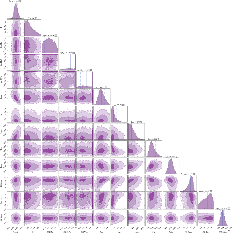
Figure 10. POSEIDON posterior distribution for visit 1. This corresponds to the simultaneous fit of the stellar contamination and planetary atmosphere for the first TRAPPIST-1 b transit (see Section 5.2).
Download figure:
Standard image High-resolution image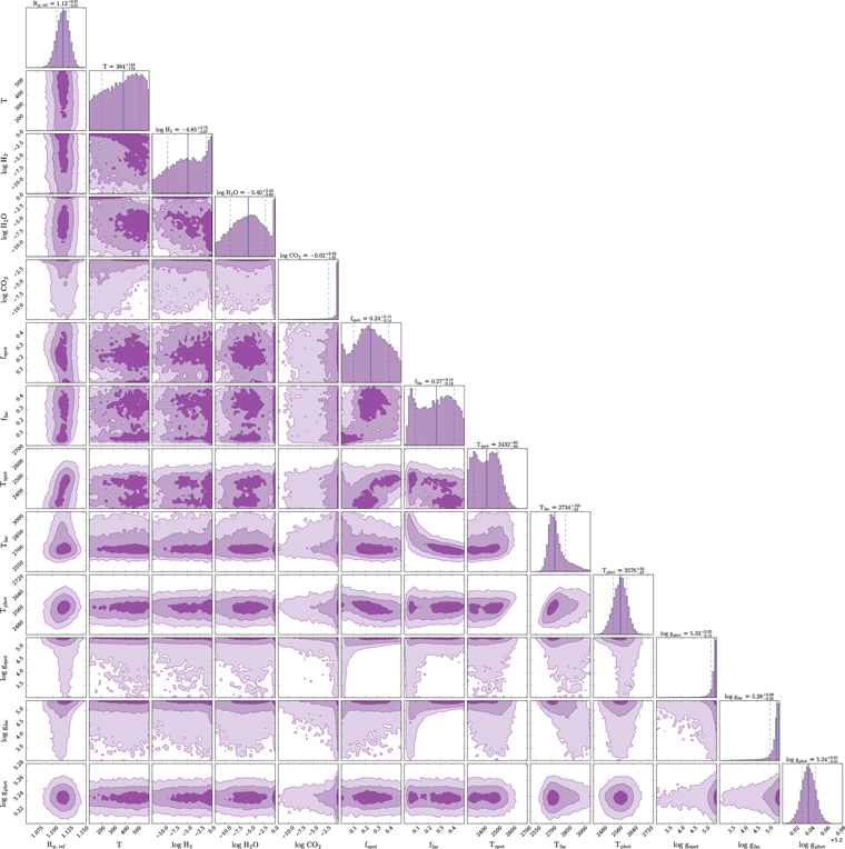
Figure 11. POSEIDON posterior distribution for visit 2. This corresponds to the simultaneous fit of the stellar contamination and planetary atmosphere for the second TRAPPIST-1 b transit (see Section 5.2).
Download figure:
Standard image High-resolution image
Footnotes
- 17
- 18
- 19
- 20
- 21
- 22
- 23
- 24
- 25
- 26
- 27
- 28
- 29
- 30