Presenting Snow Grain Size and Shape Distributions in Northern Canada Using a New Photographic Device Allowing 2D and 3D Representation of Snow Grains

Introduction

In the context of global climate change observed over the past four decades in northern regions, numerous studies have focused on the retrieval of surface state variables to monitor the rate and amplitude of observed changes (Takala et al., 2011; Brown and Derksen, 2013; Estilow et al., 2015). Globally, the rate of temperature increase has vary in the last decade (Kosaka and Xie, 2013), but Arctic air temperatures have continued to increase (+1.3°C warmer in 2015 when compared to the 1981–2010 mean) (National Oceanic and Atmospheric Administration [NOAA], 2017). Currently, the Arctic is warming at more than twice the rate of lower latitudes, leading to a decrease in sea ice cover (Serreze and Stroeve, 2015), glacier mass balance (Papasodoro et al., 2015), permafrost extent (Schuur et al., 2015) and snow cover (Derksen and Brown, 2012). This is of particular relevance in a context where snow covers up to 40 million km² during winter in North America and supports freshwater supplies for consumption, agriculture and hydroelectricity. Snow also supports a multi-billion dollar tourism and recreation industry while controlling the surface energy budget of northern ecosystems playing a crucial role on how the Earth reacts to climate change.

Numerous studies have thus focused on the retrieval of this crucial state variable over the past four decades. Pioneering work in the 1970s and 1980s (Chang et al., 1987) proposed new approaches to retrieve snow depth and water equivalent from space using passive microwave brightness temperatures. Over the years, considerable research (Foster et al., 1997; Kelly and Chang, 2003; Derksen et al., 2012; Langlois et al., 2012; King et al., 2015) has found that microwave approaches depend strongly on snow grain morphology (size and shape), which was poorly parameterized in models. This led to strong biases in the retrieval calculations (Domine et al., 2006; Langlois et al., 2010; Montpetit et al., 2012). Related uncertainties from space retrievals and the development of complex thermodynamic multilayer snow and microwave emission models motivated several studies on the development of new approaches to quantify snow grain (e.g., Domine et al., 2006; Matzl and Schneebeli, 2006; Langlois et al., 2010; Montpetit et al., 2012) given the lack of field measurements.

Until recently, grain size was poorly defined and measured, mainly due to the unstable nature of snow grain size and shape under metamorphic processes (Gallet et al., 2009). In dry conditions, snow grains can change size and shape under a temperature gradient where grain growth is observed owing to the mass transfer from warmer to colder grains, typically forming faceted and depth hoar grains (Colbeck, 1983; Gubler, 1985). In the absence of a sufficient temperature gradient (0.1 to 0.3°C/cm, Sturm et al., 2002), equilibrium metamorphism will occur where the bottom grains are at equilibrium with water vapor at a higher density than the upper grains. The high Specific Surface Area of snow (SSA), i.e., the ratio of the grain volume to its surface, then provides a lot of energy to induce microscale heat and mass transfer (e.g., Bader et al., 1939; Colbeck, 1982), changing the structure of the snow grain through a decrease in SSA (Cabanes et al., 2002). In wet conditions, the metamorphic process will change given saturated or unsaturated snow where saturated conditions will promote large grain growth from adhesion of water to the ice crystals while undersaturated conditions will lead to the formations of clusters (Denoth, 1980; Langlois and Barber, 2007).

The complexity of the thermodynamic processes involved, combined with measurement constraints, led to the development of SSA and optical diameter retrievals from optical methods. The optical diameter of snow grains can be quantified using near infrared and shortwave infrared reflectance (Kokhanovsky and Zege, 2004; Domine et al., 2006; Matzl and Schneebeli, 2006; Langlois et al., 2010; Montpetit et al., 2012) and now, measurement devices are available commercially and used by several groups. However, since such devices are expensive, traditional micro-photographs of snow grains remain widely used to “quantify” various snow grain metrics for different applications (e.g., Lesaffre et al., 1998; Langlois et al., 2007; Bartlett et al., 2008). Such photographs, if digitized, can provide interesting information and fair estimation on metamorphism processes in place but yield no information on the volume and SSA, which are key variables for microwave radiative transfer models (RTMs) (Royer et al., 2017) and retrieval approaches from space. For instance, several studies coupling RTMs with measured snow SSA for simulations of brightness temperatures have all found that a scaling factor is needed in order to optimize the difference between simulated and measured brightness temperatures (Langlois et al., 2012; Roy et al., 2013). Roy et al. (2013) hypothesized that the scaling factor is related to the grain size distribution of snow and the stickiness between grains. Even more relevant to this study is the fact that RTMs such as the Dense Media Radiative Transfer – Multi Layers (DMRT-ML) model assumes a Rayleigh snow grain size distribution (Picard et al., 2013).

Recent work has proposed innovative techniques in the measurement of SSA and correlation length. In situ techniques using near-infrared and short-wave infrared photography or shortwave infrared lasers have been rather successful, but are often cost prohibitive and very few datasets exist to date for polar snowpacks. Other well-known methods using methane absorption techniques and microCT measurements are arguably still considered as the reference methods for precise SSA measurement but are cost-prohibitive, and sample extraction for casting very large depth hoar remains extremely difficult contributing to the fact that very few research groups can build snow microstructure datasets for arctic regions. Hence, our group developed a new approach to the “traditional” measurements of snow grain metrics where micro-photographs of snow grains are taken under angular directional LED lighting. The projected shadows are digitized so that a 3D reconstruction of the snow grains is possible and distribution functions can be found for various snow grain metrics and grain types. This device, dLED (see section “Data and Methods”), has been used in several field campaigns and a very large dataset was collected and is presented in this paper. Hence, objectives of this paper are to: (1) present the low-cost dLED approach used to measure snow grain metrics, (2) provide various snow grain metric distribution functions for different grain types from over 160,000 digitized snow grains, (3) evaluate the effect of snow grain types on different snow grain metric distributions and (4) compare metrics retrieved from dLED, including the surface specific area (SSA), with well-established SSA measurements using our InfraRed Integrated Sphere (IRIS) laser-based device.

Data and Methods

Study Site

The fieldwork occurred in winter 2009–2010 for the European Space Agency “Cold Regions Hydrology high-resolution Observatory” mission concept proposal. Although the mission concept was not funded, the fieldwork allowed the collection of a very unique snow, lake ice and permafrost dataset (Derksen et al., 2012). More precisely, our field campaign was conducted in Churchill, Manitoba, Canada with logistical support from the Churchill Northern Studies Centre. The area includes forests, open areas, dry and wet fens as well as numerous lakes. The main objective of the field campaign was to acquire coincident passive and active microwave measurements over snow and lake ice, under a range of soil and vegetation conditions.

Although the field campaign included a total of six intensive observing periods from November 2009 to May 2010, this paper focuses on data collected during the four following periods: (1) January 4th–17th; (2) February 7th–20th; (3) March 14th–27th, and (4) April 18th–30th of 2010. During those short campaigns, a total of 127 snowpits were dug across wet and dry fens and forested and open areas. Of the 127 snowpits, 78 included IRIS measurements [see section “InfraRed Integrating Sphere (IRIS)”]; 107 included dLED (see section “dLED”) for a total 588 photos spanning across the four measurement periods.

Snow Measurements

dLED

The dLED was developed by our group in 2009 and consists of an enclosed box equipped of about 30 cm × 30 cm × 45 cm (first described in Royer et al., 2017), with four LEDs mounted inside on the side of the box (separated by 90°) at a height of 20 cm from the snow grain plate. They are angled at 45° in relation to the snow sample s extracted from a given layer. A Nikon D1X is mounted on top of the box and the LEDs, to take successive pictures of the illuminated grains. The Nikon D1X has a 5.0MP APS-C (23.7 cm × 15.5 mm) sized CCD sensor which provides a resolution of 3008 × 1960 pixels. A total of five pictures are taken: (1) full sample with white lighting from top (Figures 1A,B); (2) with the LED placed at azimuth 0° (Figure 1C); (3) LED at azimuth 90° (Figure 1D); (4) LED at azimuth 180° (Figure 1E), and (5) LED at azimuth 270° (Figure 1F).

Figure 1. Illustration of the different steps to compute snow grain metrics from the dLED. The two photographs at the top (A,B) represent the process of selecting a single grain, and the bottom four photographs highlight the projected shadow digitization (C–F) for a 3D reconstruction (G) of each individual grain.

In Figure 1, the grains are first digitized individually, then the projected shadows in each azimuth direction are also digitized. Once digitized, for each photo, a calibration is conducted where the 2 mm grid is digitized as scale so that the length of each pixel is known, to allow for any variability in the focus. Using the scale, the program calculates the length of each “lines” of the projected shadow in the four azimuthal directions so that the height of the snow grain’s edge creating this shadow can be calculated. As such, each 2D pixel from the initial grain digitized can be associated to a height, and a 3D representation of the snow grains is then possible. The 2D polygons are used to extract eccentricity, minor axis, major axis, projected surface and perimeter that are used in section “Snow Grains Analyzed,” of this paper. The 3D reconstruction data are used to derive SSA and compared with IRIS data in section “dLED vs. IRIS Comparison.” In both 2D and 3D cases, calculations can be done for both individual grain data, and photo averages, which in fact corresponds to a layer average. In order to avoid a user selection bias, all the snow grains from each plate (i.e., samples from a given layer) were digitized so that for the 581 photos (i.e., 581 layers), a total of 162,516 grains were digitized (averaging 263 grains digitized/photo), from which a sub-sample was manually selected for the 3D reconstruction. All metric calculations were conducted using the digitized photos. Seven snow grain metrics in total were computed:

Eccentricity

Eccentricity corresponds to the eccentricity of the ellipse that has the same second-moments as the snow grain. It considers ratio of the distance between the foci of the snow grain and its major axis length. An ellipse whose eccentricity is 0 is actually a circle, while an ellipse whose eccentricity is 1 is a line segment.

Area (mm²)

Area (mm²) computes the projected surface of the snow grain (i.e., polygon), with respect to the photograph scale. It considers the actual number of pixels in the snow grain polygon.

Minor Axis (mm)

Minor Axis (mm) corresponds to the length of the minor axis of the ellipse that has the same normalized second central moments as the snow grain polygon.

Major axis (mm)

Major axis (mm) corresponds to the length of the major axis of the ellipse that has the same normalized second central moments as the snow grain polygon.

Ratio

Ratio computed from the ratio between minor and major axes.

Perimeter (mm)

Perimeter (mm) computes the contour length of the snow grain polygon.

Equivalent sphere (mm)

Equivalent sphere (mm) diameter of a circle with the same area as the region.

With regards to the SSA retrieval precision, calibration tests using metallic bearings/balls were conducted in a laboratory, and mathematically, it can be demonstrated that the SSA derived from the projected shadows is identical to the theoretical SSA for which the rationale is presented here:

The total volume of a snow grain measured by the dLED is in fact a half-sphere, mounted on a cylinder since the projected shadows make abstraction of the curvature below the grain. In our case, the height of the cylinder is equal to the radius (r = h) with a total surface of the cylinder expressed as: 2πr² + 2πrh = 4πr² if r = h. In our case, we must subtract 1 x πr² which corresponds to the cylinder surface, located under the sphere so that we now have 3πr², and to add half the sphere surface = 4πr²/2, giving a total surface = 5πr² with an overestimation of πr².

For the volume, we simply add the cylinder volume to that of half the sphere such that: cylinder volume = πr²h = πr³ if r = h and a half sphere volume = (4/3πr³)/2 = 2/3 πr³, giving a total volume of 5/3 πr³ with an overestimation of 1/3πr³. In the context of SSA, the theoretical perfect sphere SSA can be expressed by S/V = 4πr²/4/3 πr³ = 3/r; which is identical to the SSA derived from the dLED expressed by S/V = 5πr²/5/3 πr³ = 3/r. Calibration tests using metallic sphere (steel balls from 0.8 to 4.8 mm) showed that the retrieval error (bias) on Dmax was estimated of the order of 0.03 mm.

InfraRed Integrating Sphere (IRIS)

The InfraRed Integrating Sphere (IRIS) is a laser-based device mounted on an integrating sphere collecting snow reflectance data. Based on original work from Gallet et al. (2009) (after Domine et al., 2006), who developed the first integrating sphere system for snow grain studies, our group adapted the original version for which details can be found in Montpetit et al. (2012). IRIS measures reflectance (R) at 1300 nm, which can physically be linked to SSA following the (Kokhanovsky and Zege, 2004) such that:

Where K₀ represents the escape function set at 1.26 given the geometry of the integrating sphere, which creates a mix of directional/diffuse hemispherical albedo, b a shape factor set at 4.53 that corresponds to spheres that are best described in the shortwave infrared spectrum (Picard et al., 2009) and γ_λ the absorption coefficient of ice. IRIS outputs voltages measured by a photodiode, and reflectance can be retrieved from reflectance targets measurements at 5%, 20%, 50%, 75% and 99%. This calibration is conducted for each snowpit (refer to Montpetit et al. (2012) for further details on IRIS).

Distribution Analysis

The histograms for each metric were produced for all grains considered as a whole dataset (unclassified), and separately for each grain type: (1) DF, (2) Depth Hoar (DH), (3) Facets (F), (4) Rounds (R), and (5) precipitation particles (PP). DF precipitation particles (DF) are usually found near the surface where fresh snow is broken by saltation from wind redistribution. This type of snow grain is associated with a decrease in surface area (i.e., rounding), which can lead to sintering and increase in density (Fierz et al., 2009). Depth hoar (DH) grains can be present in various forms such as striated crystals or hollows, and are typical of bottom snowpack layers formed by kinematic metamorphism under a sustained temperature gradient. Facetted snow grains (F) consist of hexagonal prisms that can be found near the surface if they develop from PP or deeper in the snowpack at early stages of DH development. Rounded grains (R) can also be found within the snow cover or near the surface and are formed from equilibrium metamorphism (within the snowpack) and by wind redistribution (near the surface). In all cases, they correspond to dense layers with an increase in strength. PP are found in numerous forms, depending on the formation process in the atmosphere driven by temperature and supersaturation levels. Their forms include dendrites, needles, plates and columns for which the rate of rounding will vary. For complete details on snow grain types, please refer to the International classification for seasonal snow on the ground (Fierz et al., 2009).

In order to select an appropriate distribution, visual diagnostics were employed to assess the quality of the fitting. We used among others, the four-parameter Kappa (KAP) distribution that has been encountered for modeling extreme hydrological values. It includes as a special case the common three-parameter distributions: generalized extremes values distribution (GEV), generalized logistic distribution (GLO), and generalized pareto distribution (GPA). The other three-parameter distributions considered are the generalized normal distribution (GNO) and Pearson type III (PE3) distribution, which, respectively, extend the common log-normal and gamma distributions with two parameters. For all these candidate distributions, the parameterization proposed by Hosking and Wallis (1997) is used, which includes a location and scale parameter, as well as 1 or 2 shape parameters, depending on the choice of the distributions. These distributions are used directly to model the snow grain metrics at the original scale, but also at the logarithm scale. The distribution of the log transformed data can be converted back to the original scale, which will be denoted, respectively, LKAP, LGEV, LGLO, LGNO, LGPA, and LPE3. Estimation is performed using L-moments (Greenwood et al., 1979; Hosking, 1992) and by removing 1% of the data (0.5% at the beginning of the distribution and 0.5% at the end) that behaves differently from the center of the distribution and has an undesirable effect on the quality of the estimation. Considering x to be the grain size, the cumulative distribution function (cdf) of the Kappa distribution can be defined as:

where ξ (location, that control the center of the distribution; central tendency), α (scale), k (shape 1), and h (shape 2) are parameters. The associated quantile function is given as:

The Kappa distribution is a generalization of some of the more commonly used three-parameter distributions: for k ≠ 0, the GPA, GEV, and GLO distributions are all special cases for h = 1, h = 0 and h = –1, respectively. The cdf, quantile function and L-moment parameter estimators for the GLO and GEV distributions can be found in Hosking and Wallis (1997) (Table 1).

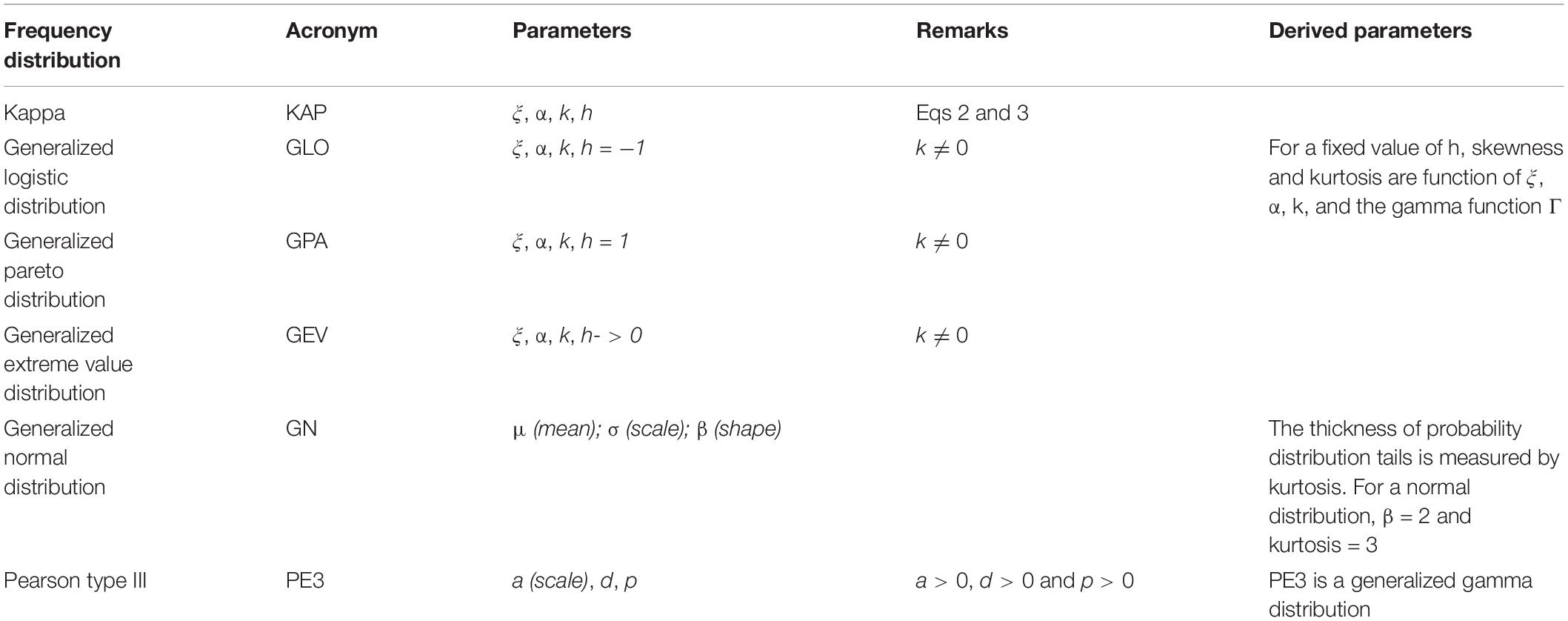
Table 1. Definition of frequency distribution used.

Results and Discussion

L-Moments Analysis

Figure 2 shows the L-moment ratio diagrams that compare the sample L-skewness and L-kurtosis to their theoretical values, which is useful to summarize their shapes. L-skewness, like classical skewness, measures asymmetry, where a positive value indicates a relatively heavier right tail compared to the left tail. Similarly, L-kurtosis is a flattening measurement where higher values correspond to relatively lower density in the center of the distribution and heavier tails. In Figure 2, sample L-moments are represented as dots. For all considered distributions except Kappa, a relationship between the L-skewness and L-kurtosis exist and takes the shape of a theoretical line as shown in Figure 2. Dots close to this theoretical line suggest good agreement between sample and theoretical L-moments. For example, in the top-left panel the black cross representing the Eccentricity metric is closer to the GEV line, which suggests this distribution as a good fit. Also, the metrics like the Major or Minor axis in the top-right panel are further from the lines, which suggests that a log-kappa that is more general maybe needed. From Figure 2, it is clear that (1) there is an appropriate distribution for each classified snow grain and (2) the distribution of each grain metric is similar for each classified snow grain.

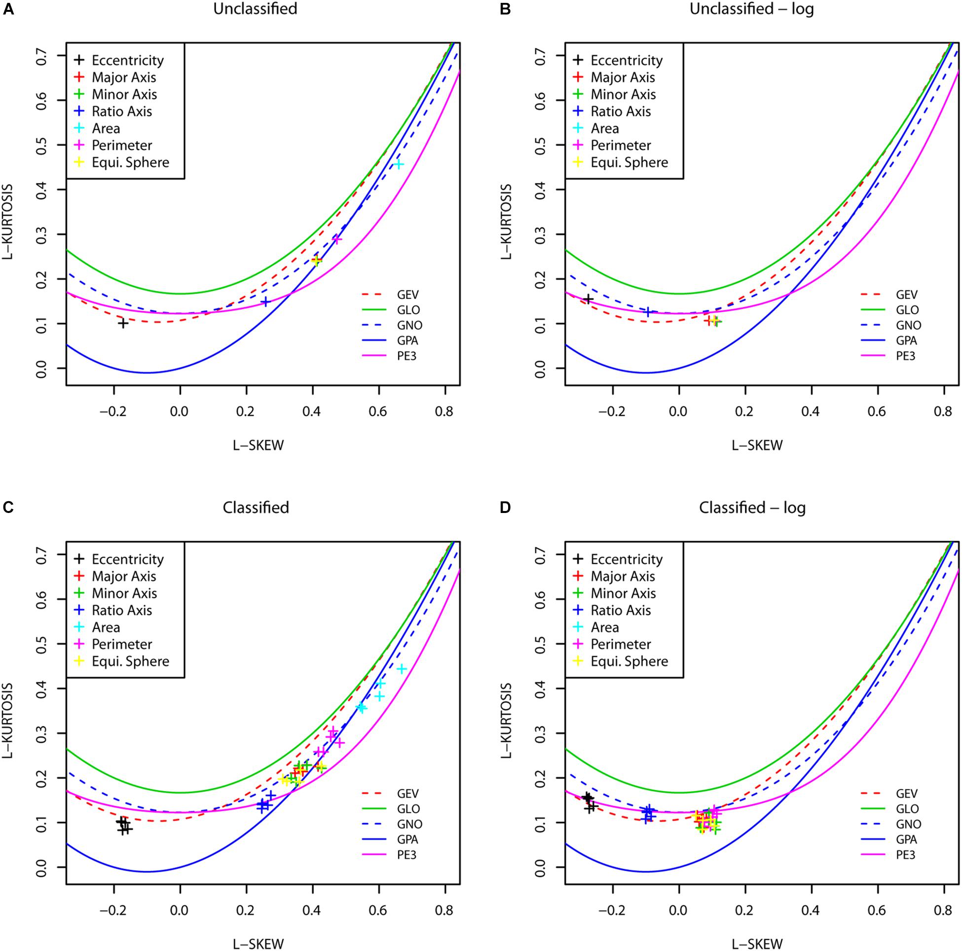
Figure 2. L-moment ratio diagrams for the unclassified snow grain dataset (A,B) (only one point for each metric) and for classified snow grains (C,D). Classified snow grains include one point for each category: Facets, Depth Hoar and Precipitation Particles. The lines represent theoretical relationship between the L-skewness and L-kurtosis of known family of distributions.

Snow Grains Analyzed

The 581 photographs were classified individually by dominant “grain type” (Fierz et al., 2009) and a total of five main classes were identified as: (1) Defragmented/broken (DF) (12,338 grains), (2) Depth Hoar (48,387 grains), (3) Facets (50,190 grains), (4) Rounds (50,633 grains), and (5) PP (967 grains). The DF grains were not used in the distribution analysis since the grains had too much visual damage to be classified. This mainly occurred in crusted layers where the insertion of the plate for the photographs was difficult. In this paper, the “unclassified” snow grain distributions correspond to the distribution analysis of the whole dataset (i.e., 162,515 snow grains), while the “classified” snow grain distributions correspond to the distribution analysis based on grain type. Also, there are many types of PP (columns, plates, dendrites and plates, hollow columns, etc.), but the distributions presented in this paper only include dendrites and plates and one should be careful when applying the distribution functions to other types of PP.

Unclassified Snow Grain Distributions

A first analysis was conducted including all digitized snow grains (i.e., 162,515 grains) so that no distinctions were made according to grain type. Distribution histograms were produced for each metric such as: eccentricity, area (projected surface 2D, mm²); minor axis (mm); major axis (mm); axis ratio (major/minor); perimeter (mm) and equivalent optical diameter (mm) and the best distribution fits were chosen from Figures 2A,B, highlighted in Figure 3 and summarized in Table 2.

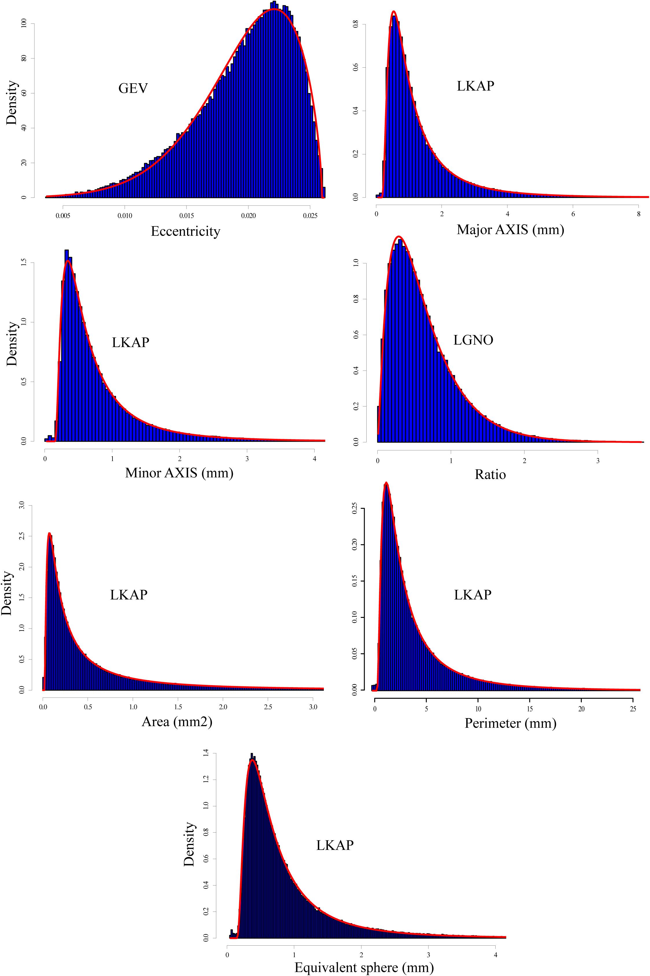
Figure 3. Snow grain metric distribution fits for all snow grains, unclassified with a total of 162,515 grains. The generalized extreme values distribution (GEV) is best for Eccentricity. The distribution of the log transformed data generalized normal distribution (LGNO) is best for Ratio while the log transformed four-parameter Kappa (LKAP) function fits Major/minor axis (mm), Area (mm²), and equivalent sphere (mm).

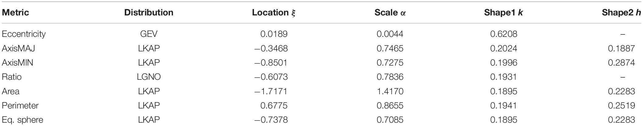
Table 2. Statistical fits summary for unclassified snow grains for the distribution of the log transformed data.

Classified Snow Grain Distributions

As mentioned earlier, the 581 photos were classified into grain “types.” Four classes are highlighted here where a distribution fit was identified for each class (Figures 4–7 and Table 3).

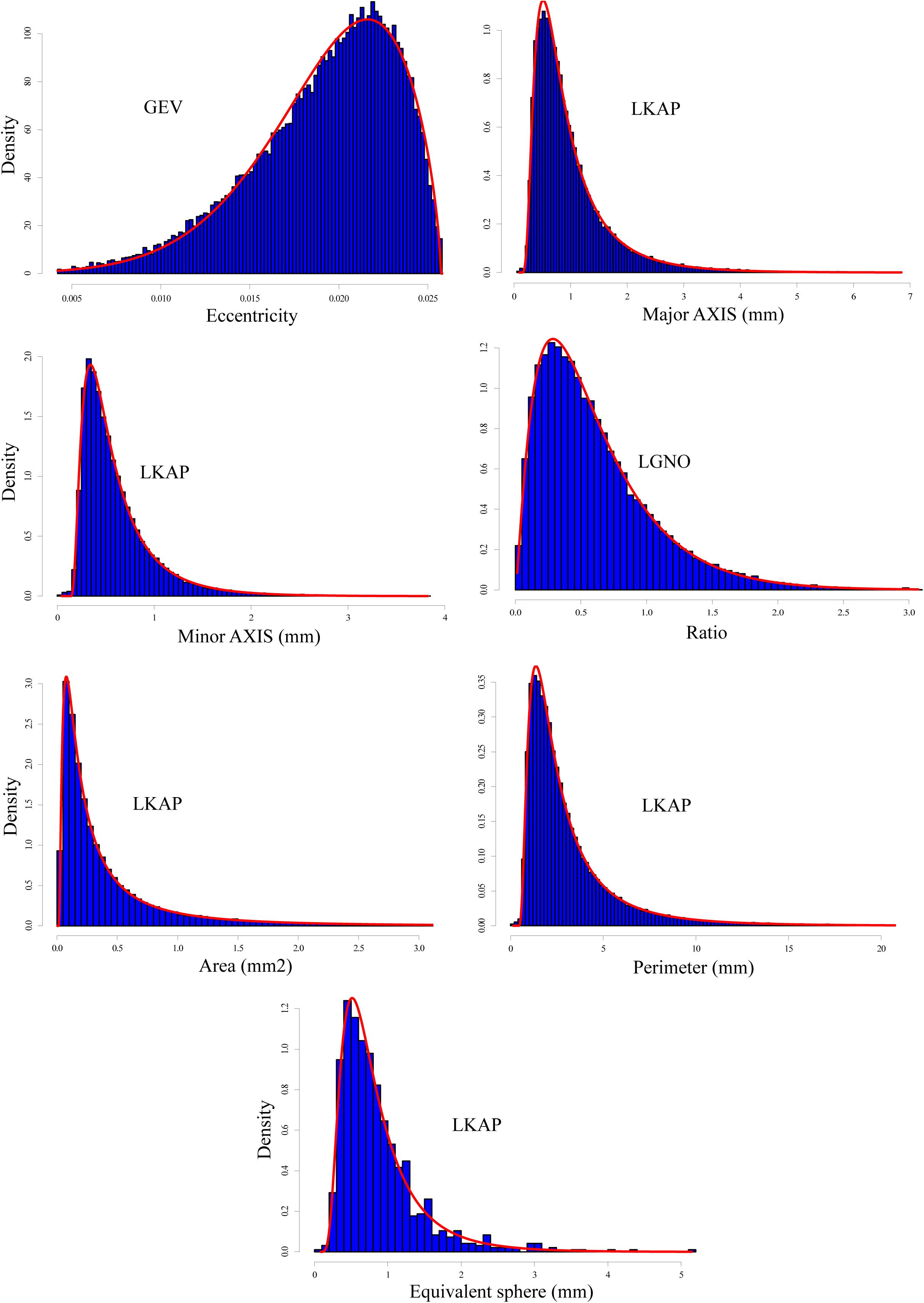
Figure 4. Same as Figure 3 but for all snow grains classified as “rounded” with a total of 50,633 grains.

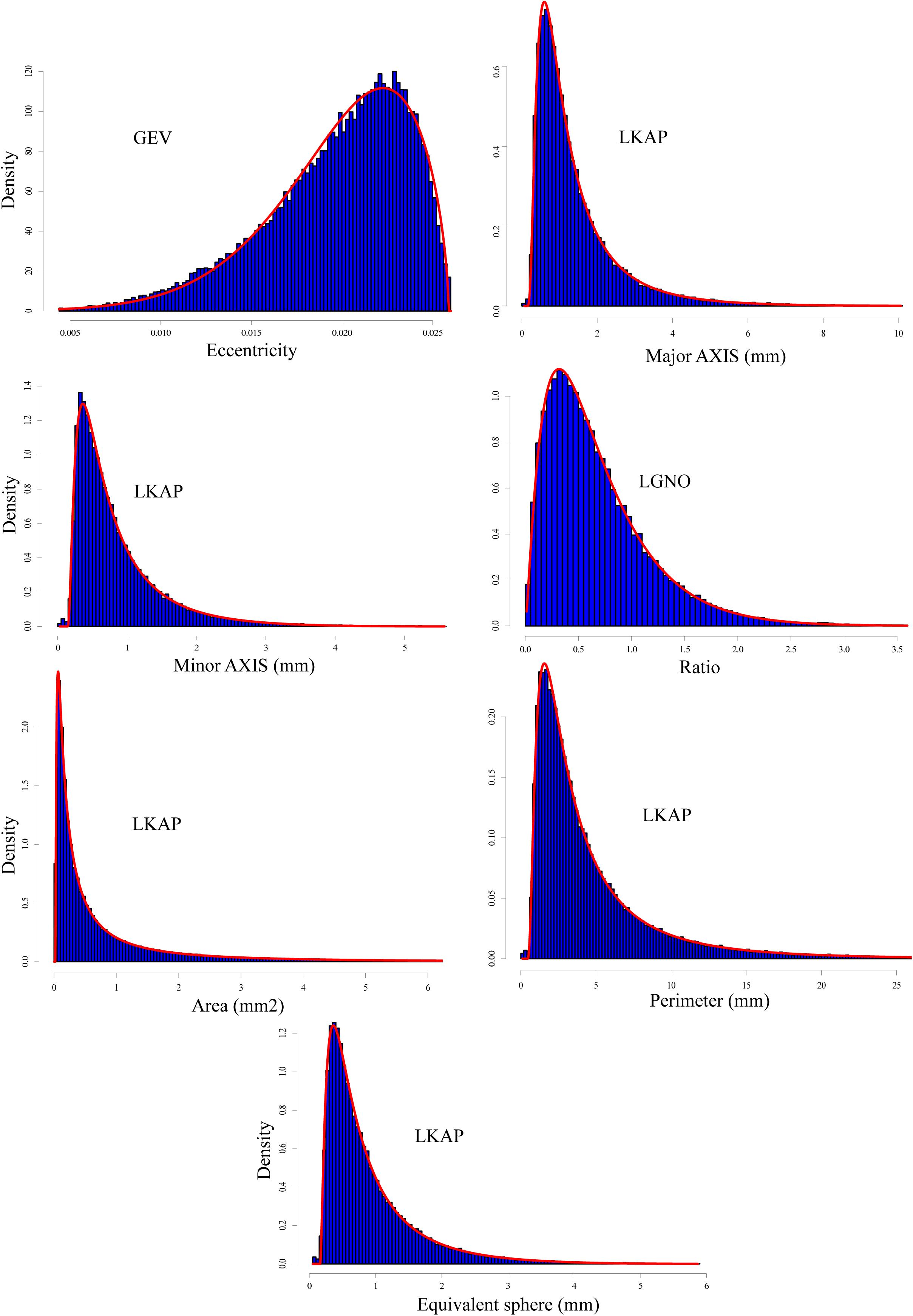
Figure 5. Same as Figure 3 but for all snow grains classified as “facetted” with a total of 50,190 grains.

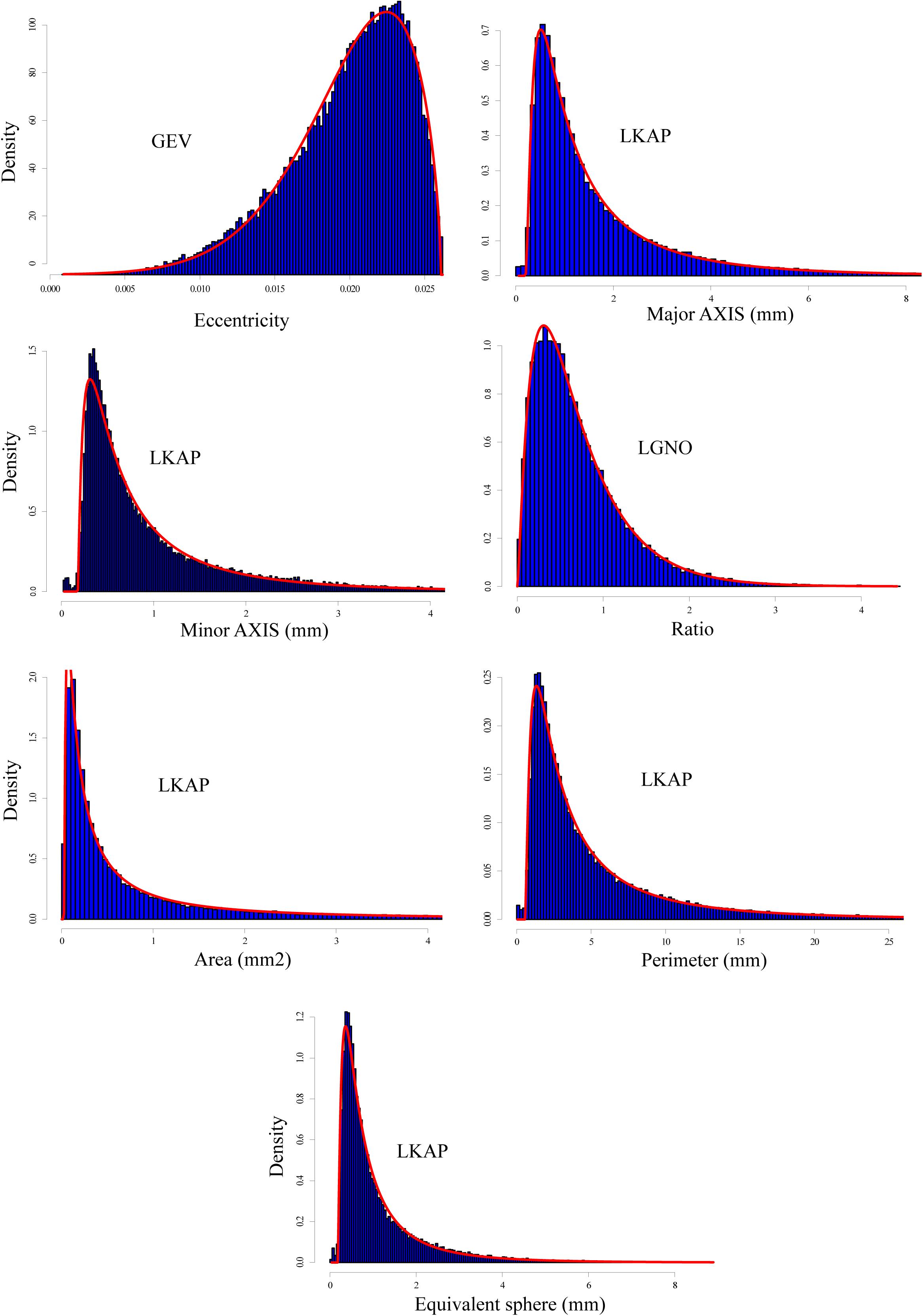
Figure 6. Same as Figure 3 but for all snow grains classified as “depth hoar” with a total of 48,387 grains.

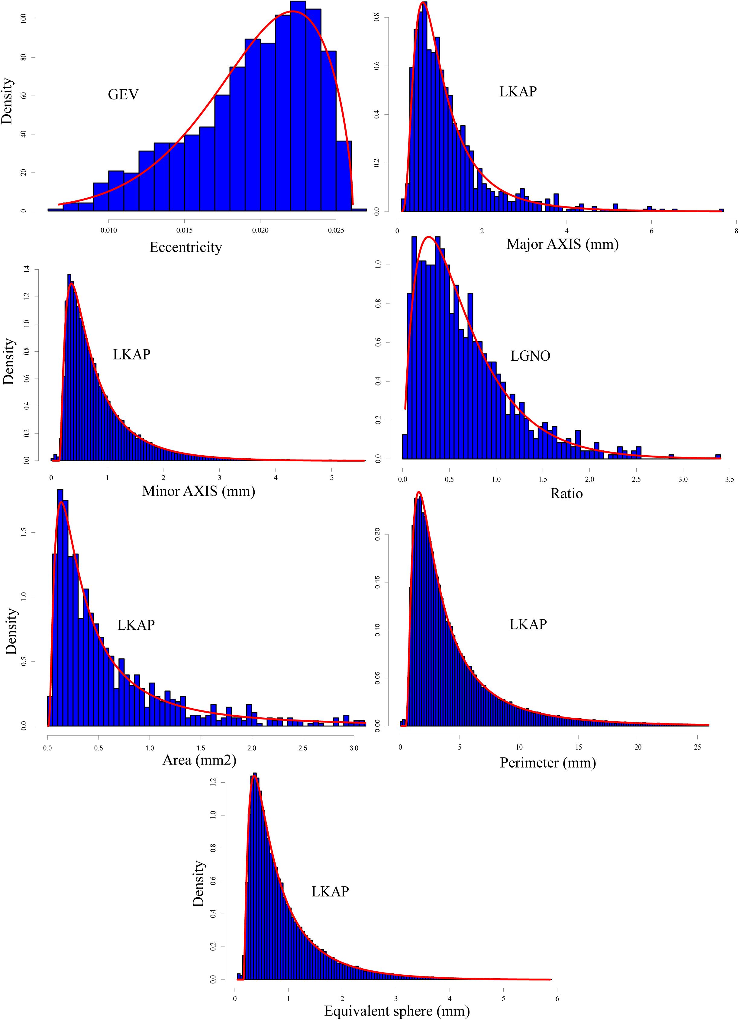
Figure 7. Same as Figure 3 but for all snow grains classified as “precipitation particles” with a total of 967 grains.

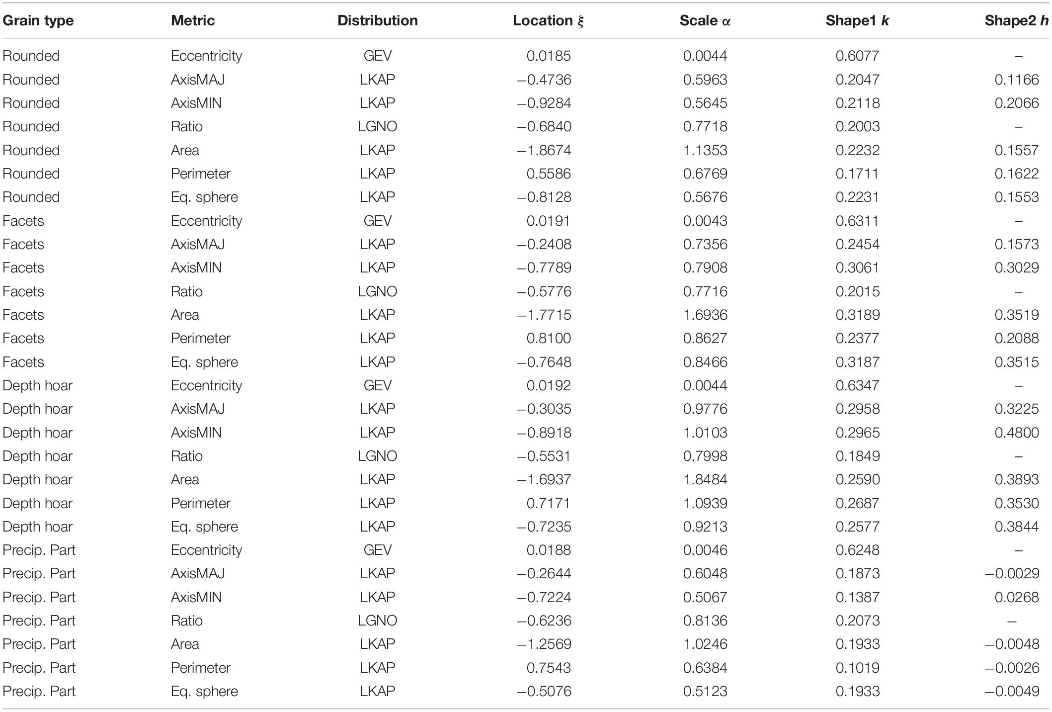
Table 3. Statistical fits summary for classified snow grains for the distribution of the log transformed data.

From Figures 4–7, we compiled the average metric statistics for the classified snow grains. The results are depicted in Table 4:

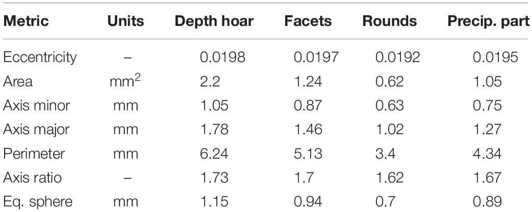
Table 4. Snow metric averages for depth hoar, facets, rounds, and precipitation particles.

From the table above, the metamorphic processes behind the formation of depth hoar are such that large snow grain are found due to the upward migration of vapor following a temperature gradient (Colbeck, 1989). Consequently, snow grain eccentricity is expected to increase as snow grains get longer. Furthermore, the area, perimeter and both minor and major axes are expected to be larger, which is the case in Table 4. Interestingly, the difference between facets and depth hoar is more marked in the “size” metrics (i.e., area, perimeter, axes and equivalent sphere) than in the shape metrics (i.e., ratio and eccentricity). When we look at rounded grains (rounds), again the changes in eccentricity and axis ratio are not as significant as changes in the “size” metrics. The rounded grains are the consequence of equilibrium metamorphism (or melt, although not the case in this study) where the large grains are eroded by a mass redistribution from the snow grain’s convex areas to its concave areas with lower saturation vapor pressure values. This process, along with significant sublimation in the absence of a temperature gradient, will lead to small and rounder grains, in agreement with the numbers presented in Table 4. Finally, PP have shape metrics similar to those of depth hoar and facets. As mentioned above, in our study, only 967 snow grains from two photographs were identified as PP. Looking at the pictures, the PP mainly consisted of flakes and a couple of needles that increased the values of eccentricity and axis ratio, but of smaller size (about 50% of area, and 25% in equivalent diameter, minor and major axes). Given what is presented, it is suggested that the size metrics present more important changes than the shape metrics from one grain type to another. However, one should note that more precipitation particle types should be considered. Fresh particles can consist of snowflakes, needles or columns, depending on the atmospheric conditions in which they formed (temperature, vapor pressure) (St-Pierre and Thériault, 2015), and considering their shape metrics individually would greatly affect the numbers presented in Table 4.

dLED vs. IRIS Comparison

Snow grain metrics from the dLED are compared to SSA measurements from the IRIS system in order to evaluate if the latter can provide information on snow grain shape. First, SSA measurements were compared to the two “shape” metrics, namely eccentricity and computed axis ratio (Figure 8).

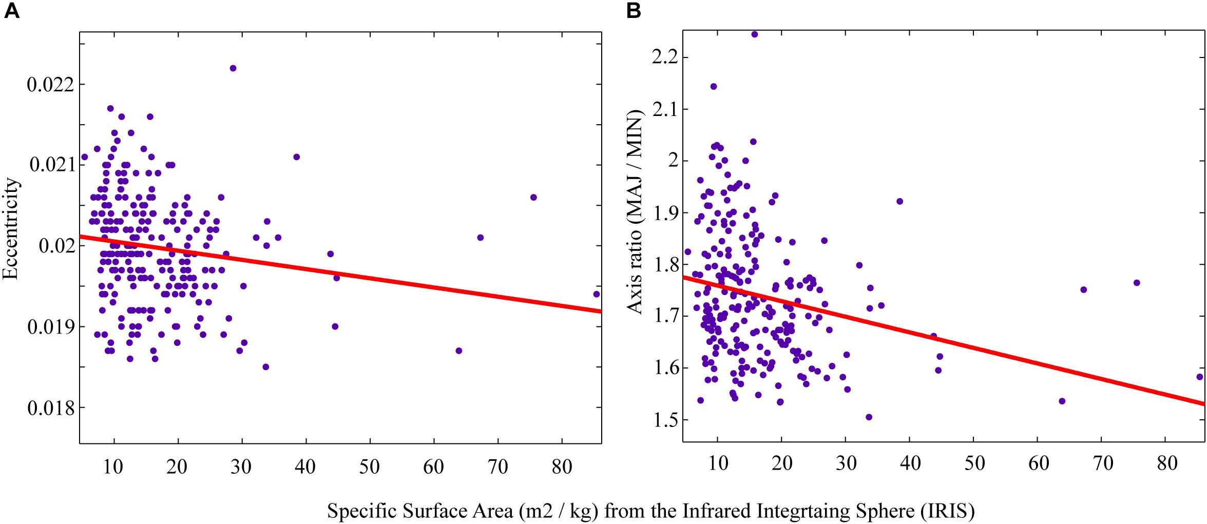
Figure 8. Measured SSA values compared with (A) eccentricity and (B) axis ratio computed from the dLED.

The comparison between IRIS SSA measurements and computed grain shape metrics did not show any statistically significant correlation. The highest correlations (although not significant) were obtained using a linear regression, with an important scatter centered around SSA values of 10 to 15 m²/kg. However, the decrease in either eccentricity and/or axis ratio with increasing SSA makes sense since an eccentricity of 0 corresponds to a perfect sphere. Therefore, for large grains such as depth hoar, the expected eccentricity would increase, whereas SSA values are usually very low for such grains. In our case, small eroded grains (rounded) would also correspond to low SSA, but would have low eccentricity. Therefore, since our dataset is mostly comprised of both grain types, it is not surprising to see that no statistical relationship can be found when comparing both. One should note, however, that the high SSA values in Figure 8 correspond to PP, which were primarily digitized as circles since the camera resolution did not produce the level of detail needed to properly draw the complicated contours of such grains. As a consequence, they are associated with low eccentricity values. The statistical fitting results are depicted in Figure 9.

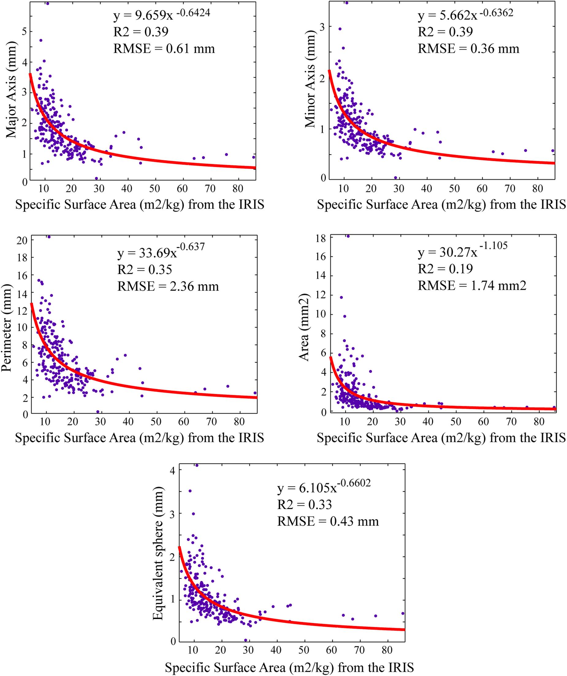
Figure 9. Measured SSA values compared with: Major axis, Minor axis, Perimeter, Area, and Equivalent sphere computed from the dLED.

The comparison between measured SSA from the IRIS and size metrics computed from the dLED highlights stronger correlations when compared to the shape metrics analysis from Figure 9. The strongest correlations are found with an exponent function, with best results obtained with minor and major axes, where the major axis can be considered, and the geometrical diameter (Langlois et al., 2010; maximum snow grain extent).

The 3D reconstruction allowed the retrieval of volume and surface for the grains so that SSA could be computed. We thus compared the computed SSA from the dLED to the IRIS in order to see if proper SSA values could be retrieved considering that the IRIS remains the best approach for SSA measurements on the field. The comparison is depicted in Figure 10 for the whole dataset, and for a measured (from IRIS) range of SSA values between 0 and 30 m²/kg.

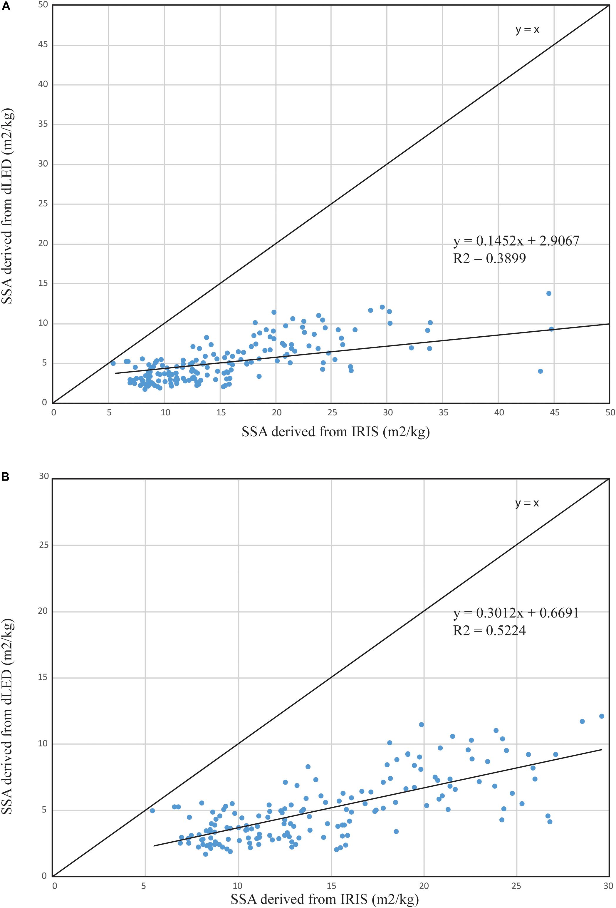
Figure 10. Comparison between specific surface area (SSA) measured with both IRIS and dLED for (A) the whole dataset and (B) measured over the value range of 0–30 m²/kg from IRIS (considered here as the reference).

Results from Figure 10 suggest an underestimation of SSA values derived from the dLED. Although statistically significant, the relationship seems to saturate for measured SSA above 30 m²/kg. The resolution of the camera and the digitization approach are such that high SSA snow grains (i.e., fresh snowflakes) are thin and complex to digitize. The projected shadows are very small so that large uncertainties can be found with such types of grains. In Figure 10A, this can be seen for SSA values above 30 m²/kg where no statistical relationship can be found. When considering values in the range of measured SSA from 0 to 30 m²/kg in Figure 10B, the correlation improves with an R² of 0.52. The underestimation remains, but results suggest that for lower SSA snow grains (i.e., easier to digitize with clear shadows), the dLED could retrieve SSA with reasonable accuracy.

Discussion

Past studies have investigated the use of snow micro-photographs to quantify various metrics (Lesaffre et al., 1998; Langlois et al., 2007, Langlois et al., 2008; Royer et al., 2017). The purpose of our study was not to overcome 2D techniques, but rather to use a new technique that allows digitizing a sufficient amount of grain to produce statistical distributions on various metrics of interests for radiative transfer models. Past works were mainly limited by the number of grains (sample size) digitized. Digitizing few snow grains per sample will lead to a user selection bias, which is avoided in our context where all shapes present in the photos are considered, and likely located in the tails of the distribution fits presented.

One limitation for this study resides in the definition of what constitutes a snow grain, which is a matter of ongoing debate in the snow community. From snow grain photographs, we must digitize snow grains as polygons, but one should note that bonded grains were not separated manually. This would have been necessary in refrozen crusts, or depth hoar chains, which were not observed in our dataset from the nature of the snow and the climate. Likely some depth hoar chains might have been broken if present by extracting the sample, but that brings us back to the definition of what constitutes a “grain.” This is an ongoing debate, especially in the metamorphism and energy exchange formulations in future snow models. This said, from a RTM perspective, we must quantify a “scatterer”, so that the proposed method in this paper remains relevant. As far as identifying the snow grains, they were manually digitized by four trained users that were asked to digitize every polygon visible on each photograph to avoid a “selection bias.” This represents several months, full time for four trained people, but we believed this was necessary to overcome limitations of past studies identified earlier. However, the authors acknowledge that this will lead to the digitization of broken grains but again, we are confident that by digitizing several hundred snow grains the contribution of broken grains will not affect the averaged metric values. Such grains would be located in the tails of the statistical distributions, thus not affecting the distribution types.

Conclusion

The work presented a very large dataset of >160,000 digitized snow grains including depth hoar, facets, rounded, and PP. The dataset was collected over a period of 6 months using a new device allowing the digitization of projected snow grain shadows under LED illumination. The use of the dLED allows the analysis and retrieval of both shape (eccentricity, axis ratio) and metric (area, perimeter, diameter, axis length) information. We analyzed various distribution functions of the classified snow grains (i.e., depth hoar, rounded, facets, and PP) and showed that the Kappa distribution function provided the best fit to the derived distributions from the dLED. More specifically, when considering all the snow grains independently from the type, the snow grain metric distributions can be explained using GEV (eccentricity), LGNO (ratio), and LKAP (minor/major axes, area, perimeter and equivalent sphere). When the snow grains are classified by type, the same distribution functions are found for each metric, but with different location, scale and shape values provided in the Tables in section “Results and Discussion.” This suggests that the distribution function with a snow cover is not only grain type dependent but depends also on the shape/metric analyzed.

The derived morphology parameters from the dLED were compared to SSA measured by the IRIS, which was considered as a reference in this paper. Results showed that a statistically significant relationship can be found between IRIS SSA and “metric” parameters, with strongest correlation with the axis lengths. This suggests that the dLED can be used to derive snow grain metrics but does not provide any significant information on grain shape (other that the ability to visually identify grain types). Furthermore, we investigated the potential in using the dLED to derive SSA from the computed volume and surface of the digitized 3D grains. Results showed that the dLED SSA are underestimated compared to the IRIS values, which can be linked to an overestimation of snow grain volume by the dLED. Although the comparison between dLED and IRIS SSA is statistically significant, the correlation improves when considering a shorter range of SSA between 0 and 30 m²/kg. In that range, the linear correlation has an R² value of 0.52. The dLED SSA remain underestimated, but in that range it can be suggested that the dLED allows SSA (mostly rounds, and depth hoar) to be derived.

This paper thus suggests distribution functions that are reproducible, and therefore useful in RTMs. The distributions found in this paper can be implemented in RTMs such as the Snow Microwave Radiative Transfer model (Picard et al., 2018) and to evaluate the improvement in simulations of brightness temperatures and the sensitivity of scaling factors to different snow grain metrics that could help assess the stickiness effect on the simulation biases. Improvements to RTMs will help improve the monitoring of snow state variables in space and time with the coupling of such models to snow thermodynamic models such as SNOWPACK (Langlois et al., 2012) or Crocus (Larue et al., 2018). For instance, SWE retrievals are critical in understanding changes in hydrological patterns at various scales. Other potential approaches using assimilation schemes to derive snow density with more accuracy will contribute largely in quantifying trends in ungulates foraging conditions that are currently endangered from snow densification (Langlois et al., 2017; Dolant et al., 2018). This is of particular relevance with the new MEaSUREs Calibrated Enhanced-Resolution Passive Microwave dataset recently available at 3.125 and 6.5 km spatial resolution (Brodzik et al., 2018), which will help produce improved maps of snow state variables at the watershed scale.

Data Availability Statement

The datasets generated for this study are available on request to the corresponding author.

Author Contributions

AL and AAR conducted the snow grain analysis, and supervised the dataset digitization, classification/distribution, and fieldwork. AL wrote the manuscript and led the manuscript analysis. AAR designed the data collection, distribution analysis, and dLED. BM performed the dataset analysis and digitization of snow grains, and contributed to the IRIS analysis. AER contributed to the microwave context, fieldwork, and data collection as well as distribution analysis on the manuscript. MD contributed to the statistical and distribution analysis. All authors reviewed the manuscript.

Funding

This work was funded by the Natural Sciences and Engineering Research Council of Canada (NSERC), the International Polar Year, and the Cold Regions H2O mission, Environment and Climate Change Canada.

Conflict of Interest

The authors declare that the research was conducted in the absence of any commercial or financial relationships that could be construed as a potential conflict of interest.

Acknowledgments

The authors would like to thank the Churchill Northern Studies Centre for tremendous logistical support during fieldwork. Special thanks to Miroslav Chum for designing the dLED and to Roxanne Lanoix for great support in digitizing the snow grain photos.

References

Bader, H. P., Haefeli, R., Bucher, E., Neher, J., Eckel, O., Tharms, C., et al. (1939). Snow and its metamorphism. U. S. Army Corps Eng. Snow Ice Permafr. Res. Establishment Transl. 14:313.
Bartlett, S. J., Rüedi, J.-D., Craig, A., and Fierz, C. (2008). Assessment of techniques for analyzing snow crystals in two dimensions. Anns. Glaciol. 48, 103–112.
Brodzik, M. J., Long, D. G., Hardman, M. A., Paget, A., and Armstrong, R. L. (2018). MEaSUREs Calibrated Enhanced-Resolution Passive Microwave Daily EASE-Grid 2.0 Brightness Temperature ESDR, Version 1. Boulder, CO: National Snow and Ice Data Center. Digital Media, doi: 10.5067/MEASURES/CRYOSPHERE/NSIDC-0630.001
Brown, R., and Derksen, C. (2013). Is Eurasian October snow cover increasing? Environ. Res. Lett. 8:024006. doi: 10.1088/1748-9326/8/2/024006
Cabanes, A., Legagneux, L., and Domine, F. (2002). Evolution of the specific surface area and of crystal morphology of Arctic fresh snow during the ALERT 2000 campaign. Atmos. Environ. 36, 2767–2777.
Chang, A. T. C., Foster, J. L., and Hall, D. K. (1987). Nimbus 7 derived global snow cover parameters. Ann. Glaciol. 9, 39–44.
Colbeck, S. C. (1989). On the micrometeorology of surface hoar growth on snow in mountainous area. Boundary Layer Meteorol. 44, 1–12.
Derksen, C., and Brown, R. (2012). Spring snow cover extent reductions in the 2008-2012 period exceeding climate model projections. Geophys. Res. Lett. 39:L19504.
Derksen, C., Smith, S. L., Sharp, M., Brown, L., Howell, S., Copland, L. et al. (2012). Variability and change in the canadian cryosphere. Clim. Change 115, 59–88. doi: 10.1007/s10584-012-0470-0
Dolant, C., Montpetit, B., Langlois, A., Brucker, L., Zolina, O., Johnson, C.-A., et al. (2018). Assessment of the Barren Ground caribou die-off during winter 2015-2016 using passive microwave observations. Geophy. Res. Lett. 45, 4908–4916. doi: 10.1029/2017GL076752
Domine, F., Salvatori, R., Legagneux, L., Salzano, R., Fily, M., and Casacchia, R. (2006). Correlation between the specific surface area and the short wave infrared (SWIR) reflectance of snow. Cold Reg. Sci. Technol. 46, 60–68.
Estilow, T. W., Young, A. H., and Robinson, D. A. (2015). A long-term Northern Hemisphere snow cover extent data record for climate studies and monitoring. Earth Syst. Sci. Data. 7, 137–142.
Fierz, C., Armstrong, R. L., Durand, Y., Etchevers, P., Greene, E., McClung, D. M., et al. (2009). The International Classification for Seasonal Snow on the Ground. International Association of Cryospheric Sciences-IACS, SC.2009/WS/15. Paris: UNESCO-IHP
Foster, J. L., Chang, A. T. C., and Hall, D. K. (1997). Comparison of snow mass estimates from a prototype passive microwave snow algorithm, a revised algorithm and a snow depth climatology. Remote Sens. Environ. 62, 132–142.
Gallet, J.-C., Domine, F., Zender, C. S., and Picard, G. (2009). Rapid and accurate measurement of the specific surface area of snow using infrared reflectance at 1310 and 1550 nm. Cryosphere 3, 167–189.
Greenwood, J. A., Lanwehr, J. M., Matalas, N. C., and Wallis, J. R. (1979). Probability weighted moments: definition and relation to parameters of several distributions expressable in inverse form. Water Resour. Res. 15, 1049–1054.
Gubler, H. (1985). Model for dry snow metamorphism by interparticle vapor flux. J. Geophys. Res. 90, 8081–8092.
Hosking, J. R. M. (1992). Moments or L moments? An example comparing two measures of distributional shape. Am. Stat. 46, 186–189.
Hosking, J. R. M., and Wallis, J. R. (1997). Regional Frequency Analysis: An Approach Based on L-moments. Cambridge: Cambridge University Press.
Kelly, R. E. J., and Chang, A. T. C. (2003). Development of a passive microwave global snow depth retrieval algorithm for SSM/I and AMSR-E data. Radio Sci. 38:8076. doi: 10.1029/2002RS002648
King, J., Kelly, R., Kasurak, A., Duguay, C., Gunn, G., Rutter, N., et al. (2015). Spatio-temporal influence of tundra snow properties on Ku-band (17.2GHz) backscatter. J. Glac. 61, 267–279.
Kosaka, Y., and Xie, S.-P. (2013). Recent global-warming hiatus tied to equatorial Pacific surface cooling. Nature 501, 403–407. doi: 10.1038/nature12534
Langlois, A., and Barber, D. G. (2007). Passive microwave remote sensing of seasonal snow covered sea ice. Prog. Phys. Geogr. 31, 539–573.
Langlois, A., Fisico, T., Barber, D. G., and Papakyriakou, T. N. (2008). Response of snow thermophysical processes to the passage of a polar low-pressure system and its impact on in situ passive microwave radiometry: a case study. J. Geophys. Res. 113:C03S04. doi: 10.1029/2007JC004197
Langlois, A., Johnson, C.-A., Montpetit, B., Royer, A., Blukacz-Richards, E. A., Neave, E., et al. (2017). Detection of rain-on-snow (ROS) events and ice layer formation using passive microwave radiometry: a context for the Peary caribou habitat in the Canadian arctic. Rem. Sens. Environ. 189, 84–95.
Langlois, A., Mundy, C. J., and Barber, D. G. (2007). Overwintering evolution of geophysical and electrical properties of snow cover over first-year sea ice. Hydrol. Proc. 21, 705–716. doi: 10.1002/hyp.6407
Langlois, A., Royer, A., Derksen, C., Montpetit, B., Dupont, F., and Goita, K. (2012). Coupling of the snow thermodynamic model SNOWPACK with the Microwave Emission Model for Layered Snowpacks (MEMLS) for subarctic and arctic Snow Water Equivalent retrievals. Water Resour. Res. 48:W12524.
Langlois, A., Royer, A., Montpetit, B., Picard, G., Brucker, L., Arnaud, L., et al. (2010). On the relationship between measured and modeled snow grain morphology using infrared reflectance. Cold Reg. Sci. Technol. 61, 34–42.
Larue, F., Royer, A., De Séve, D., Roy, A., Picard, G., and Vionnet, V. (2018). Simulation and assimilation of passive microwave data using a snowpack model coupled to a calibrated radiative transfer model over Northeastern Canada. Water Resour. Res. 54, 4823–4848. doi: 10.1029/2017WR022132
Lesaffre, B., Pougatch, E., and Martin, E. (1998). Objective determination of snow-grain characteristics from images. Anns. Glaciol. 26, 112–118.
Matzl, M., and Schneebeli, M. (2006). Areal measurement of specific surface area in snow profiles by near infrared reflectivity. J. Glac. 52, 558–564.
Montpetit, B., Royer, A., Langlois, A., Cliche, P., Roy, A., Champollion, N., et al. (2012). New short wave infrared albedo measurements for snow specific surface area retrieval. J. Glac. 58, 941–952. doi: 10.3189/2012JoG11j248
National Oceanic and Atmospheric Administration [NOAA], (2017). Global Climate Report - Annual, 2017. Silver Spring, MD: NOAA.
Papasodoro, C., Berthier, E., Royer, A., Zdanowic, C., and Langlois, A. (2015). Area, elevation and mass changes of the two southernmost ice caps of the Canadian Arctic Archipelago between 1952 and 2014. Cryosphere 9, 1535–1550.
Picard, G., Arnaud, L., Domine, F., and Fily, M. (2009). Determining snow specific surface area from near-infrared reflectance measurements: numerical study of the influence of grain shape. Cold Reg. Sci. Technol. 56, 10–17.
Picard, G., Brucker, L., Roy, A., Dupont, F., Fily, M., Royer, A., and Harlow, C. (2013). Simulation of the microwave emission of multi-layered snowpacks using the Dense Media Radiative transfer theory: the DMRT-ML model. Geosci. Model Dev. 6, 1061–1078. doi: 10.5194/gmd-6-1061-2013
Picard, G., Sandells, M., and Löwe, H. (2018). SMRT: an active–passive microwave radiative transfer model for snow with multiple microstructure and scattering formulations (v1.0). Geosci Model Dev. 11, 2763–2788.
Prowse, T. D., Furgal, C., Melling, H., and Smith, S. L. (2012). Variability and change in the Canadian cryosphere. Clim. Change 115, 59–88. doi: 10.1007/s10584-012-0470-0
Roy, A., Picard, G., Royer, A., Montpetit, B., Dupont, F., Langlois, A., et al. (2013). Snow brightness temperature simulations driven by measurements of the specific surface area of snow grains. IEEE TGRS 51, 4692–4704. doi: 10.1109/TGRS.2013.2250509
Royer, A., Roy, A., Montpetit, B., Saint-Jean-Rondeau, O., Picard, G., Brucker, L., et al. (2017). Comparison of commonly-used microwave radiative transfer models for snow remote sensing. Rem. Sens. Environ. 190, 247–259.
Schuur, E. A. G., McGuire, A. D., Schädel, C., Grosse, G., Harden, J. W., Hayes, D. J., et al. (2015). Climate change and the permafrost carbon feedback. Nature 520, 171–179. doi: 10.1038/nature14338
Serreze, M. C., and Stroeve, J. (2015). Arctic sea ice trends, variability and implications for seasonal ice forecasting. Philos. Trans. R. Soc. London Ser. A. 373, 20140159–20140159. doi: 10.1098/rsta.2014.0159
St-Pierre, M., and Thériault, J. M. (2015). Clarification of the water saturation represented on ice crystal growth diagrams. J. Atmos. Sci. 72, 2608–2611. doi: 10.1175/JAS-D-14-0357.1
Sturm, M., Perovich, D. K., and Holmgren, J. (2002). Thermal conductivity and heat transfer through the snow on the ice of the Beaufort Sea. J. Geophys. Res. 107:8043. doi: 10.1029/2000JC000409
Keywords: snow grain, distribution, radiative transfer modeling, microstructure, snow
Citation: Langlois A, Royer A, Montpetit B, Roy A and Durocher M (2020) Presenting Snow Grain Size and Shape Distributions in Northern Canada Using a New Photographic Device Allowing 2D and 3D Representation of Snow Grains. Front. Earth Sci. 7:347. doi: 10.3389/feart.2019.00347
Received: 24 July 2019; Accepted: 16 December 2019;
Published: 22 January 2020.
Edited by:
Melody Sandells, CORES Science and Engineering Limited, United KingdomReviewed by:
Veijo Pohjola, Uppsala University, SwedenPascal Hagenmuller, UMR 3589 Centre National de Recherches Météorologiques (CNRM), France
Jinmei Pan, Institute of Remote Sensing and Digital Earth (CAS), China
Copyright © 2020 Langlois, Royer, Montpetit, Roy and Durocher. This is an open-access article distributed under the terms of the Creative Commons Attribution License (CC BY). The use, distribution or reproduction in other forums is permitted, provided the original author(s) and the copyright owner(s) are credited and that the original publication in this journal is cited, in accordance with accepted academic practice. No use, distribution or reproduction is permitted which does not comply with these terms.
*Correspondence: Alexandre Langlois, a.langlois2@usherbrooke.ca