Interpreting the Microwave Spectra of Diatomic Molecules

Abstract

A brief review of the theory of the rigid rotor and its application to microwave spectroscopy is given. By careful selection of examples, procedures are given for the analysis of successively more complicated spectra, and the theory is extended to the harmonic nonrigid rotor and anharmonic nonrigid rotor when needed. The microwave spectra of carbon monoxide, and of some alkali halides, provide excellent examples for analysis and for student exercises.

1. Introduction

Microwave radiation corresponds to the frequency range from approximately 0.3 to 300 GHz and is important in modern satellite and cell phone communication. Microwaves lie between radio waves of lower frequency and infrared radiation of higher frequency and have a wavelength from 0.001 to 1 m [1]. Microwave spectroscopy gives information about the dipole moment and moments of inertia of a gas-phase molecule because the photon energies correspond to transitions between different rotational levels [2]. Radio telescopes can measure this radiation in space, supporting accurate estimates of the age of the universe through the cosmic microwave background, detecting the presence of small molecules in cosmic dust clouds, and inferring the presence of dark matter by measuring the rotational speed of galaxies via the hydrogen line at 21 cm. On Earth, microwave spectrometers have made their way into a few undergraduate laboratories [3,4], as have specialized computer programs for their prediction and analysis [5,6,7,8]. In some cases, Fourier-transform infrared spectrometers can be used to observe rotational bands [9]. The simplest spectra to analyze are molecules containing only two atoms. If performed correctly, very accurate bond distances, devoid of solvent or crystal packing effects, can be calculated.

2. Basic Theory

A diatomic molecule can be regarded as two masses, m₁ and m₂, separated by a distance r. If we assume that the distance r is fixed, then we refer to this as the rigid rotor approximation. This problem can be shown to be equivalent to a single mass μ rotating at the same distance r about an origin located at the center of mass of the molecule. This reduced mass μ is given as follows:

$$\mu =\frac{m_1{m}_2}{m_1+m_2}.$$

(1)

The moment of inertia of this system, I, is given by

$$I=\mu r^2.$$

(2)

The Schrödinger equation, applied to this system, gives the well-known energy levels [10]:

$$E=BJ\left(J+1\right),$$

(3)

where J is the rotational quantum number, and B is the rotational constant, given by

$$B=\frac{{\hslash }^2}{2I}=\frac{h^2}{8{\pi }^{2}I},$$

(4)

where h is Planck’s constant. The solution of the Schrödinger equation is rather tedious and is skipped in many texts [11]. The energy levels are 2J + 1-fold degenerate, corresponding to different values of a second quantum number m. The quantum numbers J and m are analogous to l and m_l discussed in the solution to the hydrogen atom, since the solution is the same. Because the selection rule for rotational transitions [12,13,14] is $\Delta J=\pm 1$, and because we normally deal with absorption (J corresponds to the lower state), the transitions are observed at

$$\Delta E=h\upsilon =2B\left(J+1\right).$$

(5)

A series of equally spaced lines, separated by 2B, should be observed. The rotational constant is often reported as a frequency (B/h, Hz) or as a wavenumber (B/hc, cm⁻¹). We shall refer to this simplest possible model (Equation (3)) as Model 0. Because B depends on the moment of inertia, and thus the mass of the atoms, different isotopologues will have different values of the rotational constant.

The above treatment is the deepest extent to which many texts treat the rotational spectroscopy of a diatomic molecule [15,16,17,18]. This simple approach does work for some diatomic molecules in which only the lowest vibrational level is significantly populated. We shall see below that the centrifugal distortion term and the vibration–rotation interaction are also needed to understand other spectra. Other texts acknowledge the existence of one [19,20] or both [10,21,22] of these terms, but without derivation. We provide these derivations below.

3. Materials and Methods

Zielinski advocates for the recreation of the laws of nature “through discovery and exploration the order that we see” [23]. We concur with this approach. The aim below is to present initially very simple spectra from the literature, followed by progressively more complicated spectra, in order to introduce concepts and tools on an as-needed basis. Microsoft Excel [24] with Solver [25] was used to analyze the spectra in each case, with the spreadsheets given as Supporting Information.

4. Results

4.1. Carbon Monoxide (CO)

The microwave spectrum of carbon monoxide was measured by Gilliam, Johnson, and Gordy [26]. Transitions were observed at 115,270.56 ± 0.25 MHz for ¹²C¹⁶O and at 110,201.1 ± 0.4 MHz for ¹³C¹⁶O (isotopically enriched to 14% ¹³C). The X-ray crystal structure of carbon monoxide gives a distance of 1.0629 Å [27,28]. Using this distance, the predicted value of 2B of the lighter isotopologue is 130,500 MHz (see Supplementary Material, Excel file CO.xlsx). The agreement between the predicted value of 2B and the observed value (to within 15%) suggests that the observed transition corresponds to J = 0→J = 1. This illustrates one method for assigning J, which is normally the first step. If we have two or more isotopologues, then we can check the isotopic assignments by comparing the ratio of the rotational constants to the inverse of the ratio of the reduced masses, assuming the bond length of the isotopologues is the same. In this case, B₁₂/B₁₃ = 1.04600, whereas μ₁₃/μ₁₂ = 1.04612. The agreement is reasonable. The bond distances are calculated to be 1.130895 Å (¹²C¹⁶O) and 1.130832 Å (¹³C¹⁶O). These differ from each other slightly because they correspond to the first vibrational state r₀, and they differ from those reported in ref. [26] because of the slightly smaller value of Planck’s constant used therein. Carbon monoxide has a longer bond length in the gas phase than in the solid.

The two pedagogical goals achieved here are (1) demonstrating the assignment of rotational quantum number J using extraspectroscopic information (XRD), and (2) confirming isotopologue assignment by comparing B ratios to μ ratios.

4.2. Alkali Halides

The alkali metal to halogen distances in the alkali halides in both the crystal and gas-phase, as measured by X-ray [29] and/or electron diffraction [30], respectively, are given in

Table 1. The MX distance in alkali halides (M = Li, Na, K, Rb, Cs; X = F, Cl, Br, I).

MX	R (Å) 1	R (Å) 4	Ratio
LiF	2.0086
LiCl	2.56477
LiBr	2.7506
LiI	3.000
NaF	2.310
NaCl	2.8203	2.51	1.124
NaBr	2.98662	2.64	1.131
NaI	3.2364	2.90	1.116
KF	2.6735
KCl	3.14647	2.79	1.128
KBr	3.3000	2.94	1.122
KI	3.53278	3.23	1.093
RbF	2.82
RbCl	3.2905	2.89	1.139
RbBr	3.427	3.06	1.120
RbI	3.671	3.26	1.126
CsF	3.004
CsCl	3.51 2	3.06	1.147
	3.5706 3		1.167
CsBr	3.7118 3	3.14	1.182
CsI	3.9549 3	3.41	1.159

¹ X-ray diffraction (NaCl-like). ² 450 °C. ³ X-ray diffraction (CsCl-like). ⁴ Electron diffraction (gas), 1000–1300 °C.

. Even though the crystal measurements are at a lower temperature, the distances are longer than the gas phase by an average of 12% for the NaCl-like structures and 17% for the CsCl-like structures. The major reason is that in the gas phase, the atoms only have one nearest neighbor, whereas in the solid, the atoms have six (NaCl-like) or eight (CsCl-like) equidistant nearest neighbors. The missing gas-phase results can be estimated for the purposes of predicting the rotational constants if needed.

4.3. Cesium Iodide (CsI)

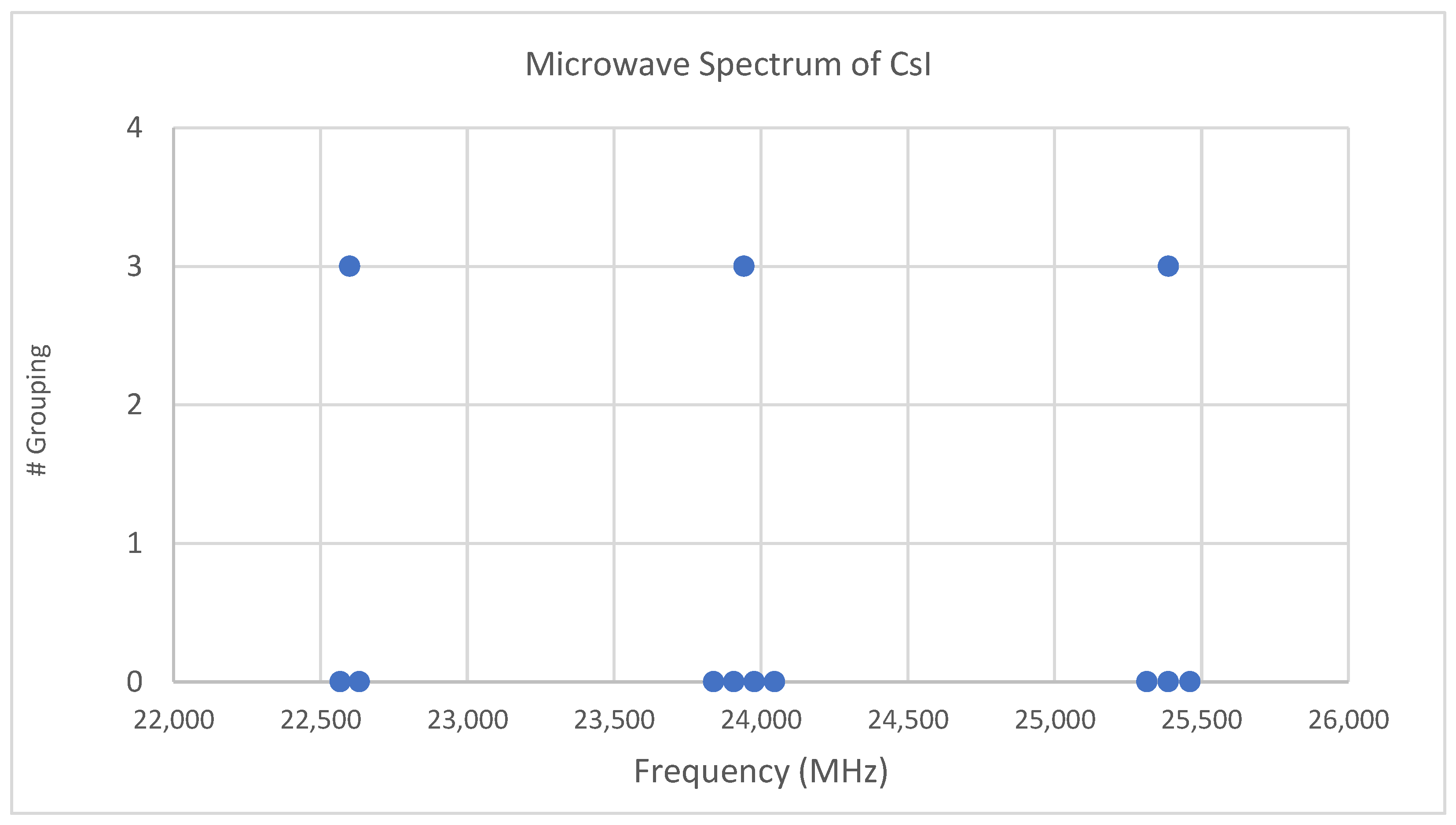
Both cesium and iodine are monoisotopic, so complications from multiple isotopologues are avoided. The predicted value of 2B from the electron diffraction value is 1340 MHz (see Supplementary Material, Excel file CsI.xlsx). The spectrum of cesium iodide in the region 22–26 GHz was measured [31] at 640 °C, and the frequencies observed (error 0.1 MHz) are given in Figure 1. Inspection of the nine frequencies (n = 9) demonstrates that there appear to be three major groupings (clusters) of frequencies. One-dimensional cluster analysis has recently been applied by the author to confirm this [32]. This tells us that the primary variation in the spectra is due to three distinct values of an independent variable, which we identify as J.

We now turn to determining J for these clusters. The cluster averages (MHz) for N = 3 are given as 22,600, 23,942, and 25,387, with differences of 1343 and 1445 (average 1394 ± 51). The predicted value of 2B is 1340 MHz, and it is therefore reasonable to assume that these clusters are due to successive values of J. The differences between the highest frequency datum (head) of each cluster are 1414.14 and 1414.13 MHz. Dividing the k = 3 cluster averages by 1340 MHz gives 16.87, 17.87, and 18.94, which suggests that these bands should be assigned as J = 16, 17, and 18, respectively. However, dividing the cluster averages by the average separation between clusters gives 16.21, 17.18, and 18.22, suggesting J = 15, 16, and 17, respectively. Dividing the heads by the head difference gives 16.00431, 17.00432, and 18.00431, which would suggest that this is the most accurate way to estimate the correct values of J + 1 (J = 15, 16, and 17).

The two pedagogical goals achieved here are (1) introducing the utility of cluster analysis, and (2) if more than one value if J is believed to be present, comparing the assignment of J using cluster averages/predicted 2B (extraspectroscopic), cluster averages/cluster differences, and head/head difference (preferred).

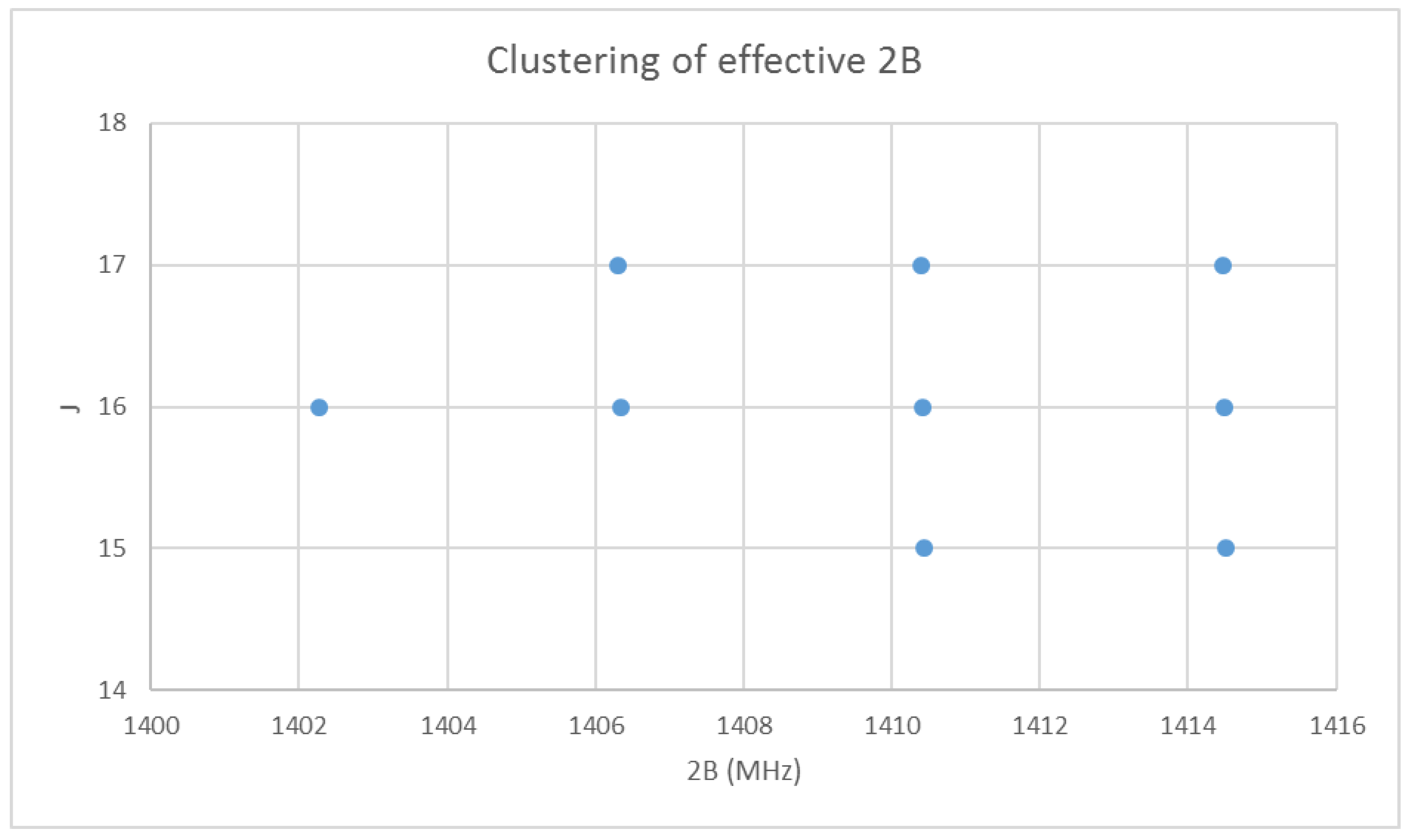
With the rotational quantum numbers J assigned, we may now calculate the effective rotational constants for each point of the spectrum. These are shown in Figure 2. The variation within each frequency cluster (or effective rotational constants) is not yet explained; however, it appears quite regular. Cluster analysis may also be carried on the effective rotational constants to show that there are four clusters [32]. There is also a very slight decrease in effective rotational constant with increasing J. We must return to the theory to explain this.

5. Advanced Theory

A diatomic molecule can vibrate as well as rotate. If the oscillation is harmonic, then for small oscillations x about the internuclear distance r_e, the Schrödinger equation is

$$-\frac{{\hslash }^2}{2\mu }\frac{d^2\psi }{d{x}^2}+\frac{1}{2}k{x}^2\psi =E\psi ,$$

(6)

where k is the spring constant. If we scale x by the constant α^1/2 to give the dimensionless ξ, where

$$\alpha ={\left(\frac{k\mu }{{\hslash }^2}\right)}^{1/2},$$

(7)

then the solutions to Equation (6) are a product of a Gaussian and a Hermite polynomial H_v:

$$\psi \left(\xi \right)=H_v\left(\xi \right)e^{-\frac{{\xi }^2}{2}},$$

(8)

where v is the vibrational quantum number [33]. The energy levels are given by

$$E_v=\hslash \omega \left(v+\frac{1}{2}\right)=h\nu \left(v+\frac{1}{2}\right),$$

(9)

where $\omega ={\left(k/\mu \right)}^{1/2}$. The energy levels of the molecule as a whole (ignoring electronic states) are the sum of the vibrational and rotational terms:

$$E_{v,J}=h\nu \left(v+\frac{1}{2}\right)+BJ\left(J+1\right).$$

(10)

If the molecule is not a harmonic oscillator, but still obeys the Born–Oppenheimer approximation, then the potential can be written as a general function $U\left(r\right)$. The Schrödinger equation can still be separated into rotational and vibrational components, and the solutions to the rotational component are still the familiar spherical harmonics. The radial equation becomes

$$\frac{1}{r^2}\frac{d}{dr}\left(r^2\frac{dR}{dr}\right)+\frac{2\mu }{{\hslash }^2}\left(E-U\left(r\right)\right)R-\frac{J\left(J+1\right)}{r^2}R=0.$$

(11)

The last term is related to the potential energy associated with a “centrifugal” force [34] due to angular momentum J. With the substitution

$$R\left(r\right)=\frac{1}{r}S\left(r\right)$$

(12)

Equation (11) may be simplified to

$$\frac{d^{2}S}{d{r}^2}+\frac{2\mu }{{\hslash }^2}\left\{E-U\left(r\right)-\frac{{\hslash }^{2}J\left(J+1\right)}{2\mu r^2}\right\}S=0.$$

(13)

If we consider a harmonic oscillator

$$U\left(r\right)=\frac{1}{2}{\left(r-r_e\right)}^2$$

(14)

then we may transform the independent variable

$$x=r-r_e,$$

(15)

and Equation (13) becomes

$$\frac{d^{2}S}{d{x}^2}+\frac{2\mu }{{\hslash }^2}\left\{E-\frac{1}{2}k{x}^2-\frac{{\hslash }^{2}J\left(J+1\right)}{2\mu {\left(r_e+x\right)}^2}\right\}S=0.$$

(16)

If x is small and can be ignored in the denominator of the last term, then Equation (16) becomes

$$\frac{d^{2}S}{d{x}^2}+\frac{2\mu }{{\hslash }^2}\left\{E-\frac{1}{2}k{x}^2-\frac{{\hslash }^{2}J\left(J+1\right)}{2\mu r_e^2}\right\}S=0.$$

(17)

This is simply the harmonic oscillator equation with the rotational energy separated out, and the energy will simply be the sum of the rotational and vibrational terms:

$$E_{v,J}=h{\nu }_e\left(v+\frac{1}{2}\right)+B_{e}J\left(J+1\right).$$

(18)

We note that the vibrational frequency ν_e and rotational constant B_e correspond to the minimum in the potential energy (the subscript e refers to equilibrium).

What happens if x becomes too large to ignore? In this case, Equation (16) is equivalent to

$$\frac{d^{2}S}{d{x}^2}+\frac{2\mu }{{\hslash }^2}\left\{E-\frac{1}{2}k{x}^2-\frac{{\hslash }^{2}J\left(J+1\right)}{2\mu r_e^2}{\left(1+\frac{x}{r_e}\right)}^{-2}\right\}S=0$$

(19)

which can be approximated, as long as $\left|x\right|<r_e$, as

$$\frac{d^{2}S}{d{x}^2}+\frac{2\mu }{{\hslash }^2}\left\{E-\frac{1}{2}k{x}^2-\frac{{\hslash }^{2}J\left(J+1\right)}{2\mu r_e^2}\left(1-2\left(\frac{x}{r_e}\right)+3{\left(\frac{x}{r_e}\right)}^2+\dots \right)\right\}S=0.$$

(20)

One way to solve this problem is by using perturbation theory on the zeroth-order harmonic oscillator equation, which we will discuss later. We examine an alternate approach. If the infinite series is truncated after the linear or quadratic terms, we obtain

$$\frac{d^{2}S}{d{x}^2}+\frac{2\mu }{{\hslash }^2}\left\{E-\frac{{\hslash }^{2}J\left(J+1\right)}{2\mu r_e^2}-\frac{1}{2}k{x}^2+\frac{2{\hslash }^{2}J\left(J+1\right)}{2\mu r_e^2}\frac{x}{r_e}\right\}S=0$$

(21)

and

$$\frac{d^{2}S}{d{x}^2}+\frac{2\mu }{{\hslash }^2}\left\{E-\frac{{\hslash }^{2}J\left(J+1\right)}{2\mu r_e^2}-\frac{1}{2}k{x}^2+\frac{2{\hslash }^{2}J\left(J+1\right)}{2\mu r_e^2}\frac{x}{r_e}-\frac{3{\hslash }^{2}J\left(J+1\right)}{2\mu r_e^2}{\left(\frac{x}{r_e}\right)}^2\right\}S=0.$$

(22)

Both of these equations are exactly soluble, because the effective potential is still quadratic. Equation (21) becomes (after rearranging and completing the square)

$$\begin{gathered} \frac{d^{2}S}{d{x}^2}+\frac{2\mu }{{\hslash }^2}\left\{E-\frac{{\hslash }^{2}J\left(J+1\right)}{2I}-\frac{1}{2}k{x}^2+\frac{2{\hslash }^{2}J\left(J+1\right)}{2I{r}_e}x\right\}S=\frac{d^{2}S}{d{x}^2}+\frac{2\mu }{{\hslash }^2}\left\{E-\frac{{\hslash }^{2}J\left(J+1\right)}{2I}-\frac{1}{2}k\left(x^2-\frac{2{\hslash }^{2}J\left(J+1\right)}{Ik{r}_e}x\right)\right\}S \\ =\frac{d^{2}S}{d{x}^2}+\frac{2\mu }{{\hslash }^2}\left\{E-\frac{{\hslash }^{2}J\left(J+1\right)}{2I}-\frac{1}{2}k\left(x^2-\frac{2{\hslash }^{2}J\left(J+1\right)}{Ik{r}_e}x+\frac{{\hslash }^4{J}^2{\left(J+1\right)}^2}{I^2{k}^2{r}_e^2}-\frac{{\hslash }^4{J}^2{\left(J+1\right)}^2}{I^2{k}^2{r}_e^2}\right)\right\}S \\ =\frac{d^{2}S}{d{x}^2}+\frac{2\mu }{{\hslash }^2}\left\{E-\frac{{\hslash }^{2}J\left(J+1\right)}{2I}+\frac{{\hslash }^4{J}^2{\left(J+1\right)}^2}{2I^{2}k{r}_e^2}-\frac{1}{2}k{\left(x-\frac{{\hslash }^{2}J\left(J+1\right)}{Ik{r}_e}\right)}^2\right\}S=0. \end{gathered}$$

(23)

If we substitute

$$y=x-{\delta }_1,{\delta }_1=\frac{{\hslash }^{2}J\left(J+1\right)}{Ik{r}_e},$$

(24)

then we obtain

$$\frac{d^{2}S}{d{y}^2}+\frac{2\mu }{{\hslash }^2}\left\{E-\frac{{\hslash }^{2}J\left(J+1\right)}{2I}+\frac{{\hslash }^4{J}^2{\left(J+1\right)}^2}{2I^{2}k{r}_e^2}-\frac{1}{2}k{y}^2\right\}S=0.$$

(25)

This is just the normal harmonic oscillator equation with usual solution, except an extra term is taken out, which is formally identified as the centrifugal distortion term [35]:

$$D{J}^2{\left(J+1\right)}^2=\frac{{\hslash }^4{J}^2{\left(J+1\right)}^2}{2I^{2}k{r}_e^2}.$$

(26)

The harmonic oscillator solutions are no longer centered about x = 0, but increase with rotational constant by δ₁.

If we now include the quadratic term as well, Equation (22) becomes

$$\frac{d^{2}S}{d{y}^2}+\frac{2\mu }{{\hslash }^2}\left\{E-\frac{{\hslash }^{2}J\left(J+1\right)}{2I}+\frac{{\hslash }^4{J}^2{\left(J+1\right)}^2}{2I^{2}k{r}_e^2}-\frac{1}{2}k{y}^2-\frac{3{\hslash }^{2}J\left(J+1\right)}{2\mu r_e^2}{\left(\frac{y+{\delta }_1}{r_e}\right)}^2\right\}S=0.$$

(27)

Expanding and collecting terms, we obtain

$$\frac{d^{2}S}{d{y}^2}+\frac{2\mu }{{\hslash }^2}\left\{E-\frac{{\hslash }^{2}J\left(J+1\right)}{2I}+\frac{{\hslash }^4{J}^2{\left(J+1\right)}^2}{2I^{2}k{r}_e^2}-\frac{1}{2}\left(k+\frac{3{\hslash }^{2}J\left(J+1\right)}{I{r}_e^2}\right)y^2-\frac{3{\hslash }^4{J}^2{\left(J+1\right)}^2}{k{I}^2{r}_e^3}y-\frac{3{\hslash }^6{J}^3{\left(J+1\right)}^3}{2k^2{I}^3{r}_e^4}\right\}S=0.$$

(28)

If we let

$$k\prime =k+\frac{3{\hslash }^{2}J\left(J+1\right)}{I{r}_e^2},$$

(29)

then

$$\begin{gathered} \frac{d^{2}S}{d{y}^2}+\frac{2\mu }{{\hslash }^2}\left\{E-\frac{{\hslash }^{2}J\left(J+1\right)}{2I}+\frac{{\hslash }^4{J}^2{\left(J+1\right)}^2}{2I^{2}k{r}_e^2}-\frac{3{\hslash }^6{J}^3{\left(J+1\right)}^3}{2k^2{I}^3{r}_e^4}-\frac{1}{2}k\prime \left(y^2+\frac{6{\hslash }^4{J}^2{\left(J+1\right)}^2}{k^{\prime }k{I}^2{r}_e^3}y+\frac{9{\hslash }^8{J}^4{\left(J+1\right)}^4}{{k^{\prime }}^2{k}^2{I}^4{r}_e^6}\right) \\ +\frac{9{\hslash }^8{J}^4{\left(J+1\right)}^4}{2k^{\prime }{k}^2{I}^4{r}_e^6}\right\}S=0. \end{gathered}$$

(30)

If we substitute

$$z=y+{\delta }_2, {\delta }_2=\frac{3{\hslash }^4{J}^2{\left(J+1\right)}^2}{k^{\prime }k{I}^2{r}_e^3}$$

(31)

then we obtain

$$\frac{d^{2}S}{d{z}^2}+\frac{2\mu }{{\hslash }^2}\left\{E-\frac{{\hslash }^{2}J\left(J+1\right)}{2I}+\frac{{\hslash }^4{J}^2{\left(J+1\right)}^2}{2I^{2}k{r}_e^2}-\frac{3{\hslash }^6{J}^3{\left(J+1\right)}^3}{2k^2{I}^3{r}_e^4}+\frac{9{\hslash }^8{J}^4{\left(J+1\right)}^4}{2k^{\prime }{k}^2{I}^4{r}_e^6}-\frac{1}{2}k\prime z^2\right\}S=0.$$

(32)

Some third- and fourth-order (in $J\left(J+1\right)$) pure rotational terms have been subtracted out, and we are left with the usual harmonic oscillator problem, but with a different force constant k′. The main effect is on the vibrational energy levels:

$$E_v=\hslash {\left(\frac{k\prime }{\mu }\right)}^{1/2}\left(v+\frac{1}{2}\right)=\hslash {\left(\frac{k}{\mu }\right)}^{1/2}{\left(1+\frac{3{\hslash }^{2}J\left(J+1\right)}{kI{r}_e^2}\right)}^{1/2}\left(v+\frac{1}{2}\right),$$

(33)

and, therefore, this effect is called the vibration–rotation interaction. It can be approximated as

$$E_v=h{\nu }_e\left(1+\frac{3{\hslash }^{2}J\left(J+1\right)}{2kI{r}_e^2}-\frac{9{\hslash }^4{J}^2{\left(J+1\right)}^2}{8k^2{I}^2{r}_e^4}+\cdots \right)\left(v+\frac{1}{2}\right)=h{\nu }_e\left(v+\frac{1}{2}\right)+h{\nu }_e\frac{3{\hslash }^2}{2kI{r}_e^2}J\left(J+1\right)\left(v+\frac{1}{2}\right)+\cdots .$$

(34)

We may let

$${\alpha }_e=h{\nu }_e\frac{3{\hslash }^2}{2kI{r}_e^2}.$$

(35)

When combined with the significant rotational terms, we obtain

$$E_{v,J}=h{\nu }_e\left(v+\frac{1}{2}\right)+B_{e}J\left(J+1\right)-D{J}^2{\left(J+1\right)}^2+{\alpha }_{e}J\left(J+1\right)\left(v+\frac{1}{2}\right).$$

(36)

If we let the effective rotational constant for vibrational level v be

$$B_v=B_e+{\alpha }_e\left(v+\frac{1}{2}\right),$$

(37)

then we can see that each vibrational level will have a different effective rotational constant, and that the effective rotational constants are approximately evenly spaced. [36] Although Equation (35) predicts that α_e is positive, in practice it is negative because of anharmonicity (below). The variation in the effective rotational constant, as seen in Figure 2, is thus explained as being due to the vibrational quantum number v.

Alternatively, we may apply perturbation theory to the harmonic oscillator, with the following perturbation:

$$H^{\left(1\right)}=\frac{{\hslash }^2}{2\mu }\frac{J\left(J+1\right)}{{\left(r_e+x\right)}^2}+\frac{1}{3!}{U}^{\left(3\right)}{x}^3+\frac{1}{4!}{U}^{\left(4\right)}{x}^4+\cdots .$$

(38)

First-order perturbation theory will have no contribution from terms of odd order in x. The first-order correction to the energy (from terms of even order in x) is

$$E_{v,J}^{\left(1\right)}=\frac{{\hslash }^2}{2I}J\left(J+1\right)+\frac{3{\hslash }^3}{2I{r}_e^2{\left(k\mu \right)}^{1/2}}J\left(J+1\right)\left(v+\frac{1}{2}\right)+\left(\frac{1}{4!}{U}^{\left(4\right)}+\frac{4{\hslash }^2}{2I{r}_e^4}J\left(J+1\right)\right)f\left(v+\frac{1}{2}\right)+\cdots .$$

(39)

where f is a quadratic function in $v+\frac{1}{2}$. The second-order correction to the energy contains the centrifugal distortion correction (from the linear term in x), a vibrational anharmonicity term involving ${\left(U^{\left(3\right)}\right)}^2{\left(v+\frac{1}{2}\right)}^2$, and additional terms involving $J\left(J+1\right){\left(v+\frac{1}{2}\right)}^j,j=1-4$ [34,37]. The j = 1 term here is usually larger than the corresponding first-order term and is opposite in sign, explaining why α_e is usually negative. The first-order correction involving the quadratic function f and the j = 2 term of the second-order correction can be related to γ_e below.

The pedagogical goal achieved here is to show what happens to the energy levels when the molecule cannot be treated as a harmonic oscillator and rigid rotor, in order to explain some of the finer structure in the spectra of alkali halides.

6. More Results

6.1. Cesium Iodide (CsI, Reprise)

Returning to Figure 2, it is now clear that the four clusters represent different vibrational states, and we assign them to $v=0-3$, with the highest frequency corresponding to $v=0$. We may either model the effective rotational constants via Equation (37), or model the rotation spectra itself using Model 1:

$$\Delta E_{v,J}=2B_e\left(J+1\right)-2{\alpha }_e\left(J+1\right)\left(v+\frac{1}{2}\right).$$

(40)

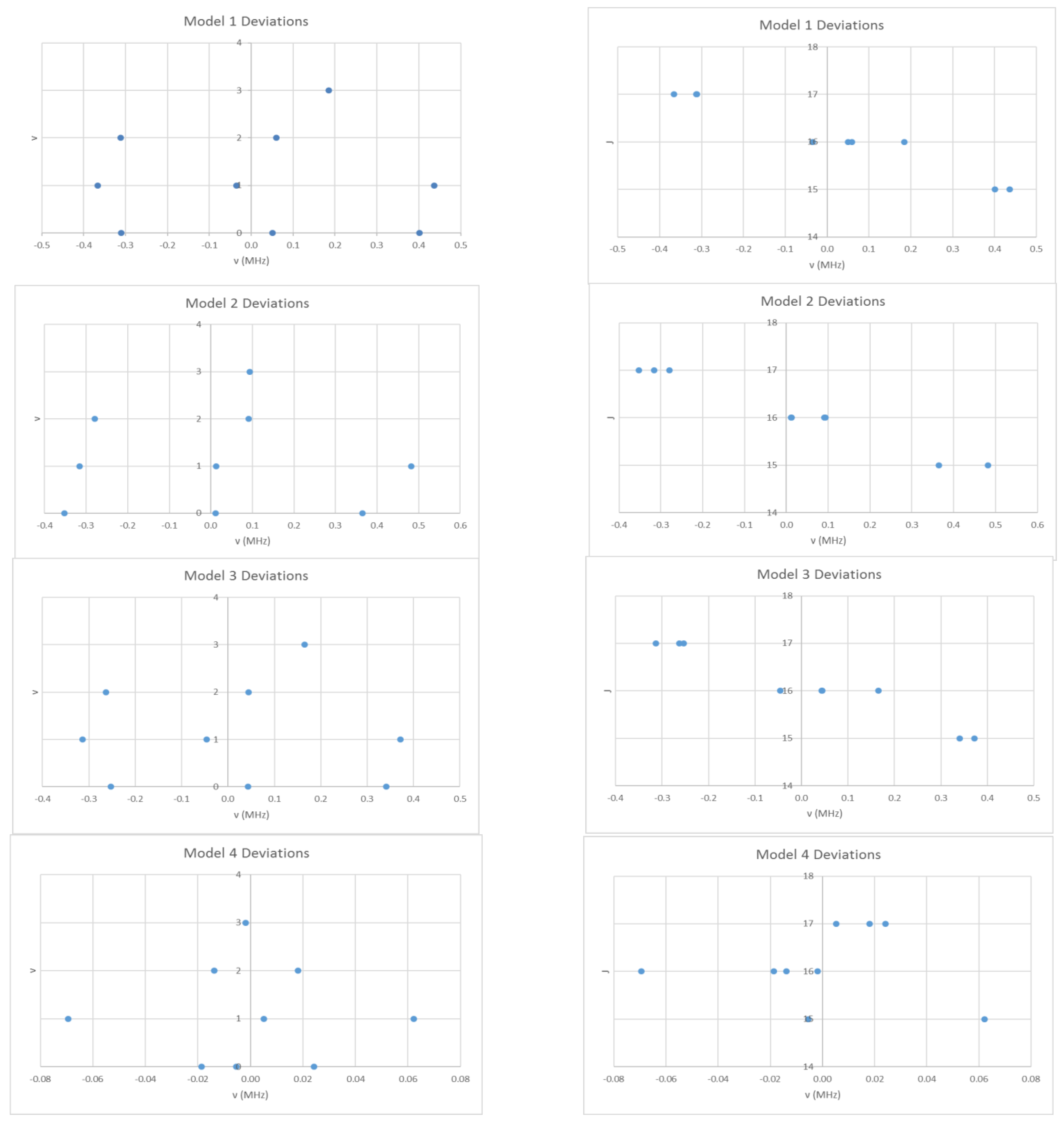
These will give slightly different results under equal weighting least squares. We obtain B_e = 708.266 and α_e = 2.040 MHz, sum of squares error (SSE) = 0.7213 (Model 1,

Table 2. Model parameters for cesium iodide (MHz) (¹³³Cs¹²⁷I, n = 9).

Model	Be	αe	γe	De1	SSE
1	708.266	2.040	n/a	n/a	0.7213
2	708.269	2.045	0.0015	n/a	0.6840
3	708.280	2.040	n/a	25.7	0.5194
4	708.362	2.043	0.0011	162	0.0102

¹ Centrifugal distortion constants have been multiplied by 10⁶.

). In Figure 3, the error in this model is plotted as a function of the quantum numbers v and J. The error is up to five times the estimated error (0.1 MHz) in each individual measurement, which suggests that improvements can be made to the model. In addition, the error appears to have a quadratic dependence on v and a linear dependence on J. Model 1 may be improved by adding a quadratic term in v + ½ to give Model 2:

$$\Delta E_{v,J}=2B_e\left(J+1\right)-2{\alpha }_e\left(J+1\right)\left(v+\frac{1}{2}\right)-2{\gamma }_e\left(J+1\right){\left(v+\frac{1}{2}\right)}^2,$$

(41)

or by adding a centrifugal distortion term to give Model 3:

$$\Delta E_{v,J}=2B_e\left(J+1\right)-2{\alpha }_e\left(J+1\right)\left(v+\frac{1}{2}\right)-2D_e{\left(J+1\right)}^3.$$

(42)

Model 2 removes the quadratic dependence of the error on v, (B_e = 708.269, α_e = 2.045, γ_e = 0.0015 MHz, SSE = 0.6840), whereas Model 3 keeps it (B_e = 708.280, α_e = 2.040, D_e = 2.57 × 10⁻⁵ MHz, SSE = 0.5194). The error is reduced to an acceptable level only by including both terms (Model 4):

$$\Delta E_{v,J}=2B_e\left(J+1\right)-2{\alpha }_e\left(J+1\right)\left(v+\frac{1}{2}\right)-2{\gamma }_e\left(J+1\right){\left(v+\frac{1}{2}\right)}^2-2D_e{\left(J+1\right)}^3,$$

(43)

which gives a much lower SSE (B_e = 708.362, α_e = 2.043, γ_e = 0.0011, D_e = 1.62 × 10⁻⁴ MHz, SSE = 0.0102). The estimated Cs-I bond distance is 3.3151 Å, which is about 0.1 Å shorter than the electron diffraction result. This microwave result corresponds to r_e, whereas the electron diffraction result would be a Boltzmann average over many vibrational and rotational states. Even so, each unit increase in vibrational quantum number adds only about 0.005 Å to r_v for CsI.

The pedagogical goals achieved here show that for CsI, (1) the most important extension to the simplest model is to include the vibrational number dependence of the effective rotational constants via Model 1, (2) they demonstrate how to assign vibrational quantum numbers, and (3) the incorporation of either the D_e and γ_e terms lead to an approximately equal (but small) reduction in error, whereas incorporation of both leads to a much better fit.

6.2. Cesium Bromide (CsBr)

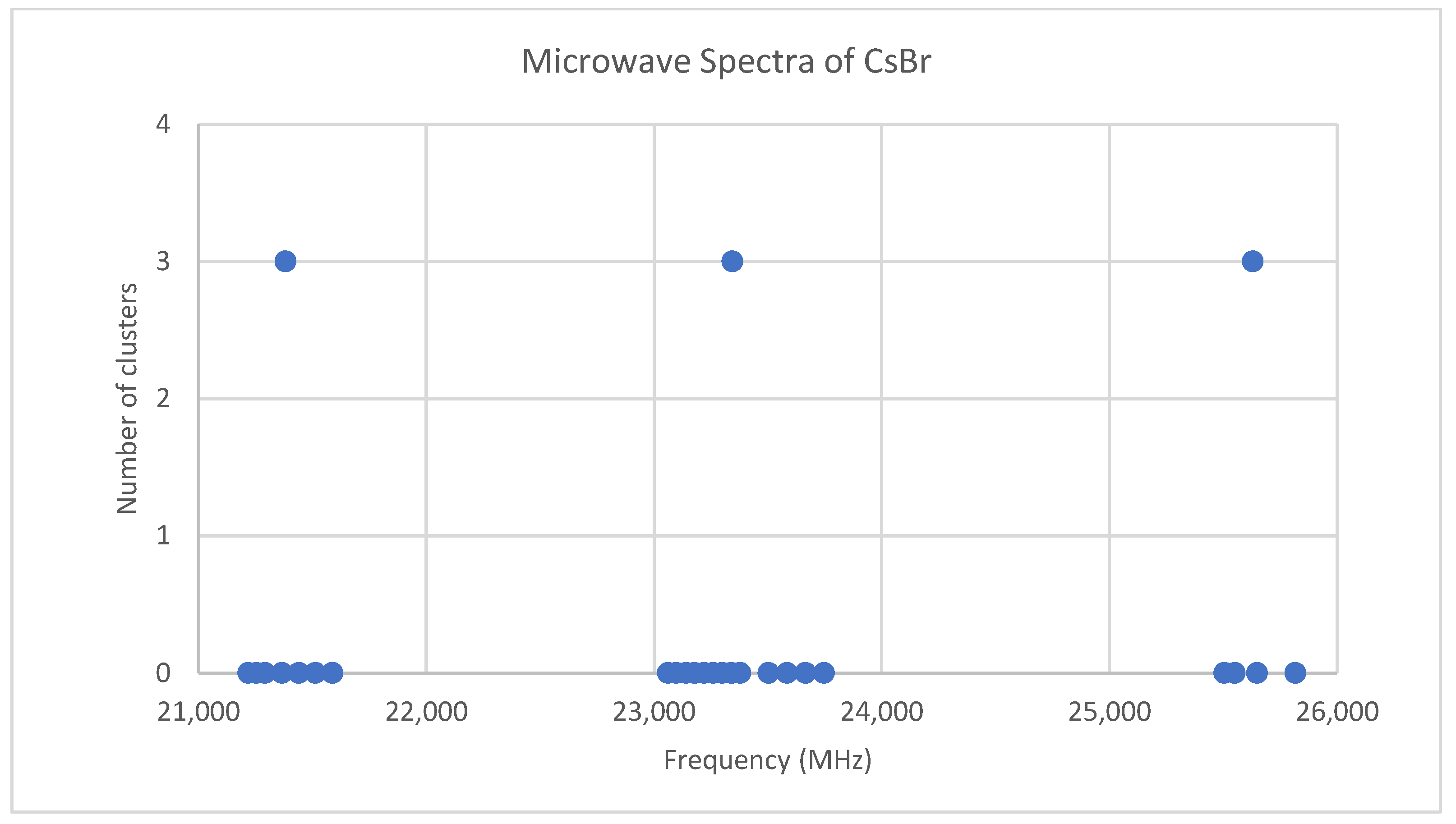
Bromine has two isotopes in approximately a 1:1 ratio, so two isotopologues should be observable in natural samples. The predicted value of 2B from the electron diffraction value is 2100 MHz (see Supplementary Material, Excel file CsBr.xlsx). The spectrum of cesium bromide in the region 21–26 GHz was measured [31] at 690 °C, and the frequencies observed (error 0.1–0.2 MHz) are given in Figure 4. Inspection of the 24 frequencies demonstrates that there are three clusters of frequencies centered at 21,382, 23,334, and 25,630 MHz [32]. The average difference of these is 2124 ± 150 MHz. The highest frequency per cluster differences is 2113 ± 45 MHz. These all suggest transitions corresponding to J = 9, 10, and 11.

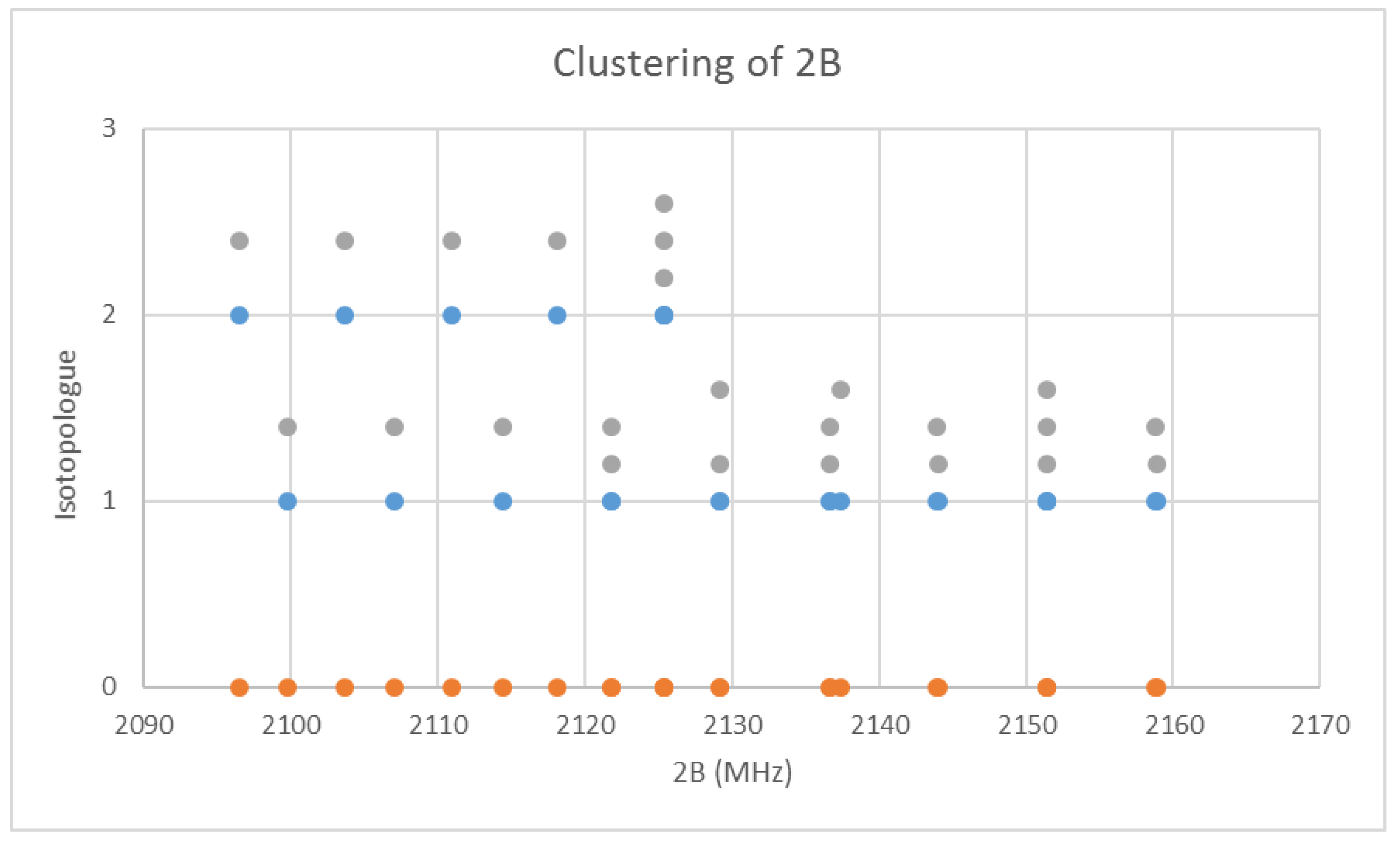
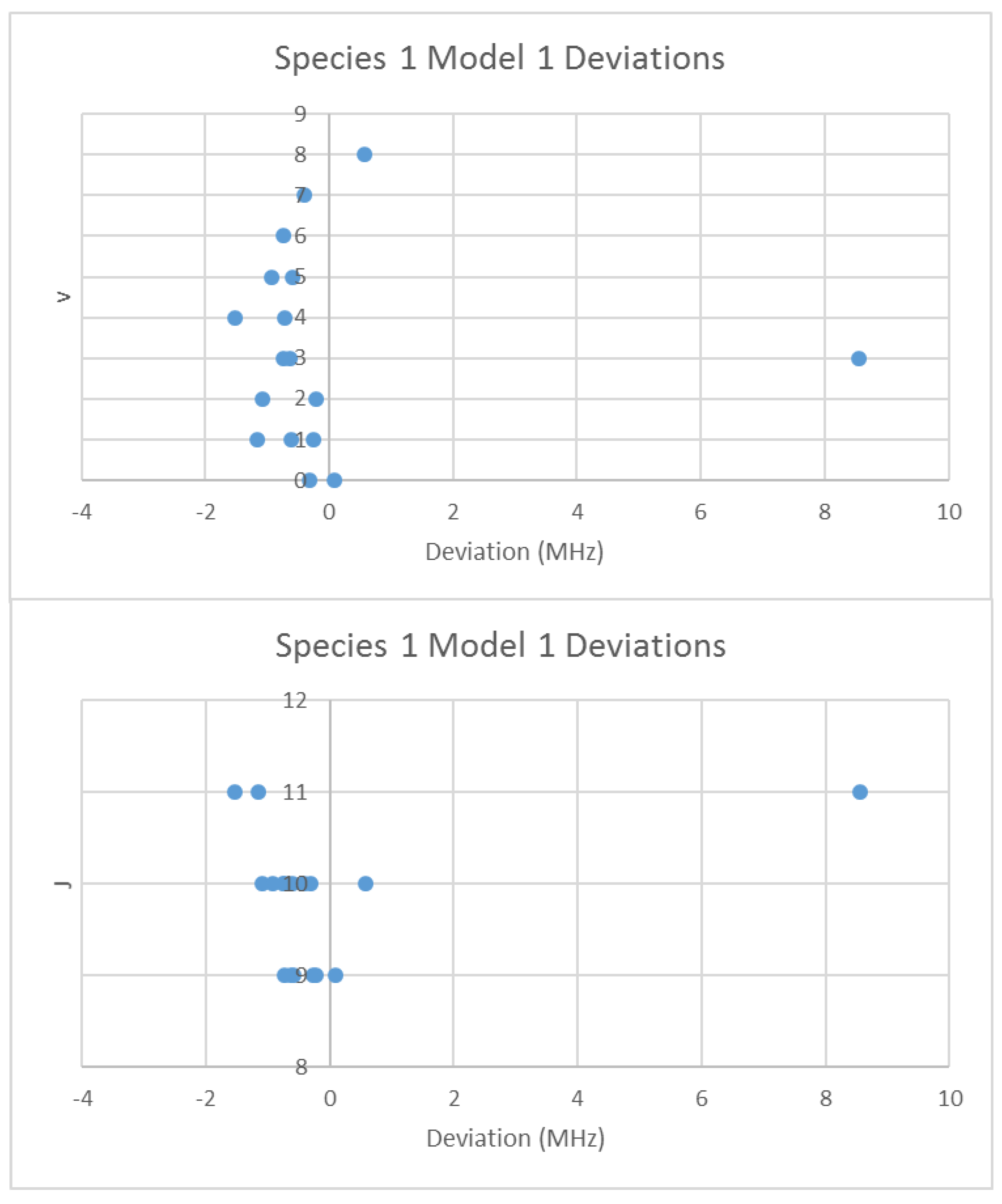
When the effective rotational constants (×2) are plotted (Figure 5), it can be seen that they naturally divide themselves into two series of equally spaced progressions, with the exception of a point at 2137.4 MHz corresponding to the observed frequency at 25,648.95 MHz. Fitting of these to Equation (37) gives B_e values of 1081.27 and 1064.51 MHz. This was performed by fitting the data to both isotopologues and choosing the smaller of the two sum-of-squared errors. The deviation in 2B for the “wrong” isotopologue is an approximately constant 33 MHz. This procedure also enables separation by isotopologue. The isotopologue mass ratio is 1.015736, and the B_e ratio is 1.015744, an agreement to five significant figures. This is strong evidence that the higher frequency progression (Isotopologue 1) is ¹³³Cs⁷⁹Br, and the lower frequency progression (Isotopologue 2) is ¹³³Cs⁸¹Br. We can analyze these progressions separately. Using Model 1, the residual error for ¹³³Cs⁷⁹Br is plotted in Figure 6. The “bad” point corresponds to v = 3, J = 11. While a Q-test on the residuals can be used to exclude this point, it is important to note that this point appears to be 10 MHz too high. We suspect that this is a printing error, and that this value should actually be 25,638.95 MHz instead of 25,648.95 MHz. We will use this value henceforth as it reduces the SSE 20-fold. The results of fitting to all four models are given in

Table 3. Model parameters for cesium bromide (MHz) (¹³³Cs⁷⁹Br, n = 17; ¹³³Cs⁸¹Br, n = 7).

	Model	Be	αe	γe	De1	SSE
133Cs79Br	1	1081.242	3.692	n/a	n/a	3.998
	2	1081.283	3.720	0.0033	n/a	1.426
	3	1081.281	3.692	n/a	−0.162	2.520
	4	1081.313	3.718	0.0030	−0.138	0.361
133Cs81Br	1	1064.512	3.617	n/a	n/a	0.263
	2	1064.521	3.632	0.0032	n/a	0.177
	3	1064.538	3.618	n/a	−0.097	0.130
	4	1064.552	3.635	0.0037	−0.107	0.018

¹ Centrifugal distortion constants have been multiplied by 10⁶.

. In all cases, the B_e ratio matches the expected isotopic mass ratio by five significant figures. For Model 4, the r_e values for the two isotopologues, 3.072274 and 3.072287 Å, are in excellent agreement.

The pedagogical goals achieved here show that for CsBr, calculating effective rotational constants using Model 1 can (1) help assign points to different isotopologues, (2) identify a “bad” point, and (3) confirm isotopologue assignments by a calculation of B_e ratios.

6.3. Cesium Chloride (CsCl)

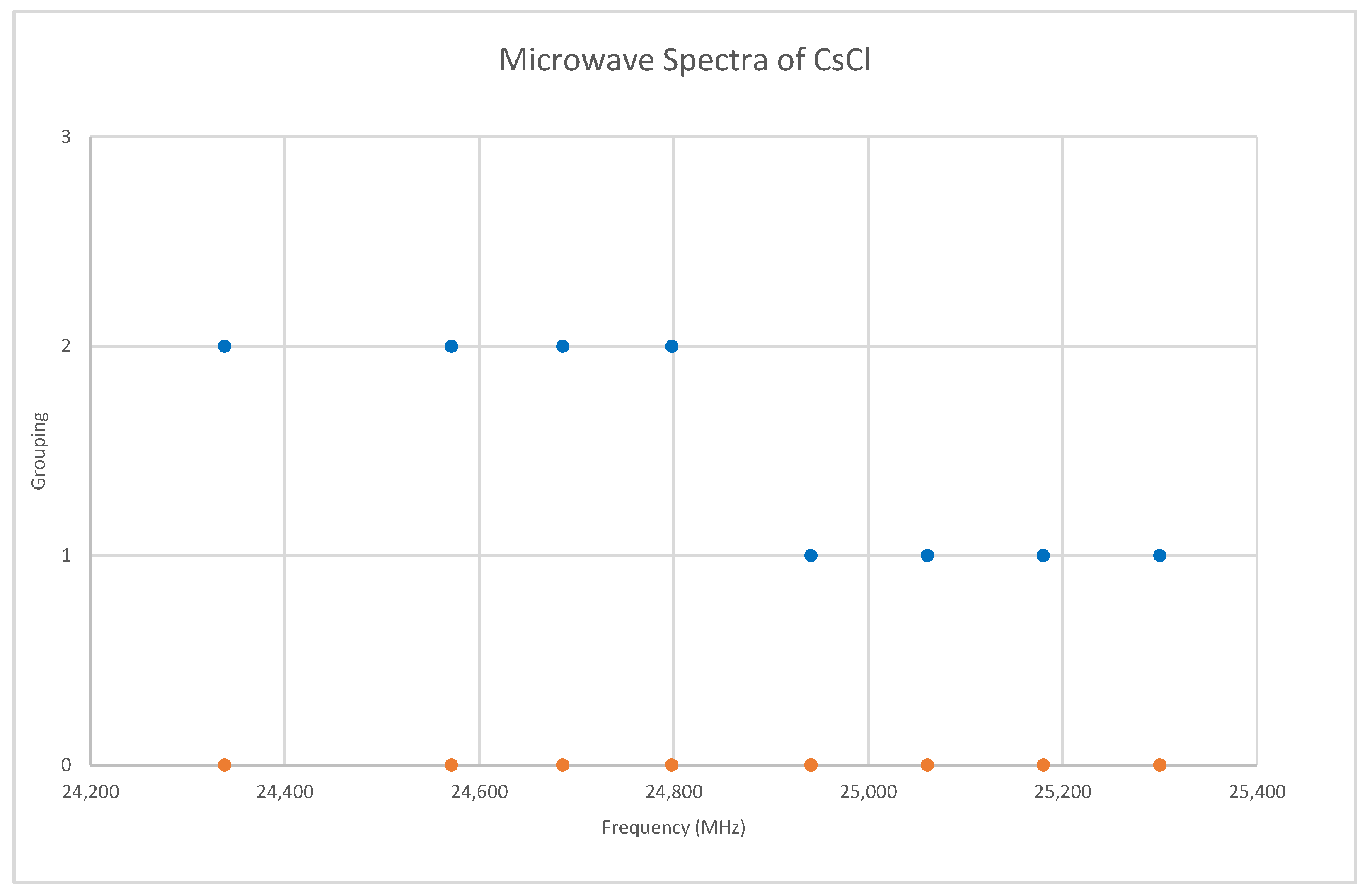
Chlorine has two isotopes in approximately a 3:1 ratio, so two isotopologues should be observable in natural samples. The predicted value of 2B from the electron diffraction value is 4000 MHz (See Supplementary Materials, Excel file CsCl.xlsx). The spectrum of cesium chloride in the region 24.3–25.4 GHz was measured [38] at 715 °C, and the frequencies observed (error 1.5 MHz) are given in Figure 7. Inspection of the eight frequencies demonstrates that there appears to be just one major grouping of frequencies. The estimated value of 2B suggests transitions corresponding to J = 5. There are two apparent gaps at about 24,450 and 24,880 MHz, which appear to be due to a missing transition and a break between two vibrational progressions, respectively. We note that because we do not have multiple values of J, there is no way to estimate the centrifugal distortion constant. We also note that the error in each measurement is fairly large compared to the previous two cesium salts analyzed.

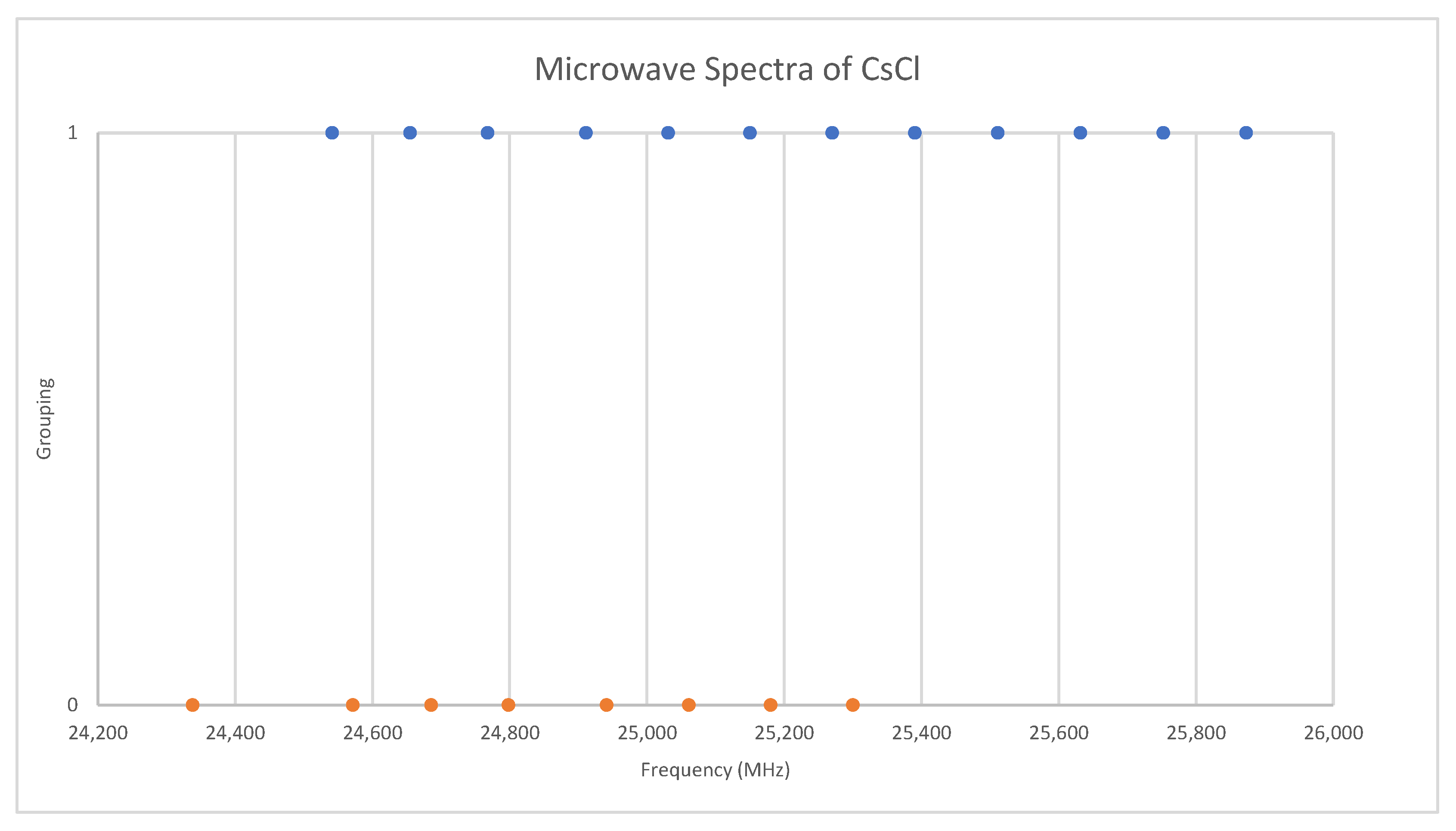
Under the assumption that the head of each progression corresponds to v = 0, we find that the higher frequency progression is well described by Model 1, with B_e = 2113.31 and α_e = 9.96, whereas the lower frequency progression gives B_e = 2071.45 and α_e = 9.60 (all MHz). The expected mass ratio is 1.04468, but the B_e ratio is 1.02020. Therefore, the vibrational assignments are incorrect, and we must revise our assumption. It is unlikely that we would miss the head of the progression of the heavier isotopologue, as it falls within the range of other observed bands, so we assume that we have assigned this correctly and that we have misassigned the lighter isotopologue because it falls out of the observed range. With this model, any misassignment of v results in the same α_e, but different B_e. The following B_e ratios are calculated for head assignments v = 1–5: 1.025, 1.029, 1.034, 1.039, and 1.044. This suggests that the assignments of the lighter isotopologue correspond to v = 5–8 instead of v = 0–3, and that the isotopologues are ¹³³Cs³⁵Cl and ¹³³Cs³⁷Cl. This was confirmed by a later measurement at 720 °C [31], where the missing transitions (v = 0–4) were seen. The newer results were all systematically lower in frequency by 30 MHz, but the precision was improved to 0.1–0.5 MHz (Figure 8). The model parameters are given in

Table 4. Model parameters for cesium chloride (MHz).

	Model	Be	αe	γe	SSE
133Cs35Cl [38], n = 4	1	2163.119	9.963	n/a	0.115
[31], n = 9	1	2161.029	10.021	n/a	4.195
	2	2161.152	10.10	0.0091	0.522
133Cs37Cl [38], n = 4	1	2071.458	9.600	n/a	8.940
	2	2071.155	9.238	−0.0703	0.002
[31], n = 3	1	2068.713	9.436	n/a	0.035
	2	2068.682	9.378	−0.0192	exact

. For Model 2, the r_e values for the two isotopologues, 2.906337 and 2.906362 Å, are in excellent agreement.

The pedagogical goal achieved here is showing that the vibrational assignments should always be checked by comparison of the predicted B_e ratios.

6.4. Cesium Fluoride (CsF)

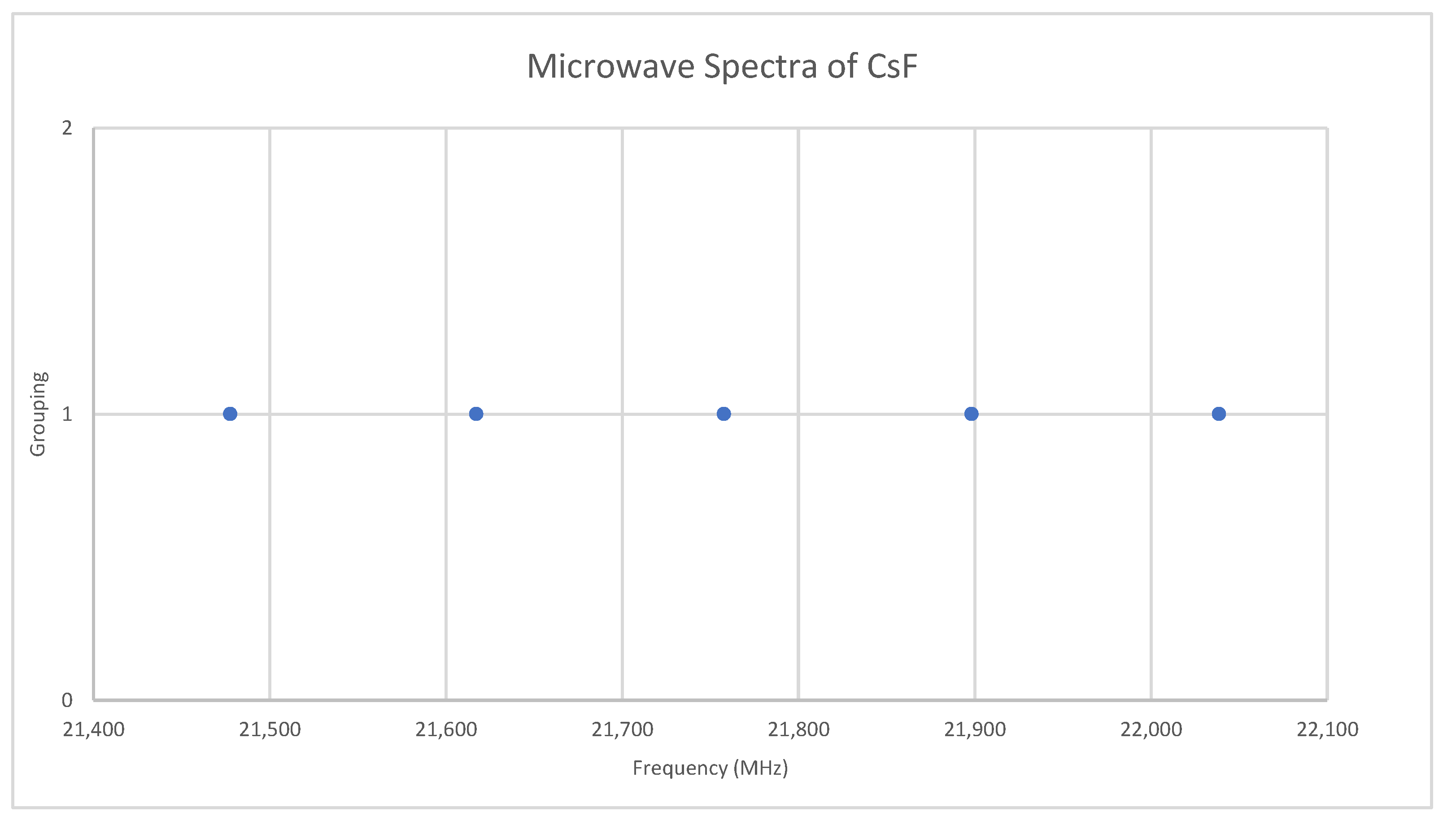
Fluorine is monoisotopic. The predicted value of 2B from the electron diffraction value is 10,000 MHz (See Supplementary Materials, Excel file CsF.xlsx). The spectra of cesium fluoride in the region 21.4–22.1 GHz was measured [31] at 700 °C, and the frequencies observed (error 0.2–1.0 MHz) are given in Figure 9. Inspection of the five frequencies demonstrates that there appears to be just one major grouping of frequencies. The observed spectrum corresponds to J = 1, v = 0–4. Fitting gives B_e = 5527.123, α_e = 35.072 (Model 1), and B_e = 5527.259, α_e = 35.218, γ_e = 0.0279 (Model 2), all MHz. The bond distance r_e is 2.3454 Å. This problem makes an excellent student exercise (Appendix A) without the complicating effects of multiple J and/or isotopes.

6.5. Rubidium Iodide (RbI)

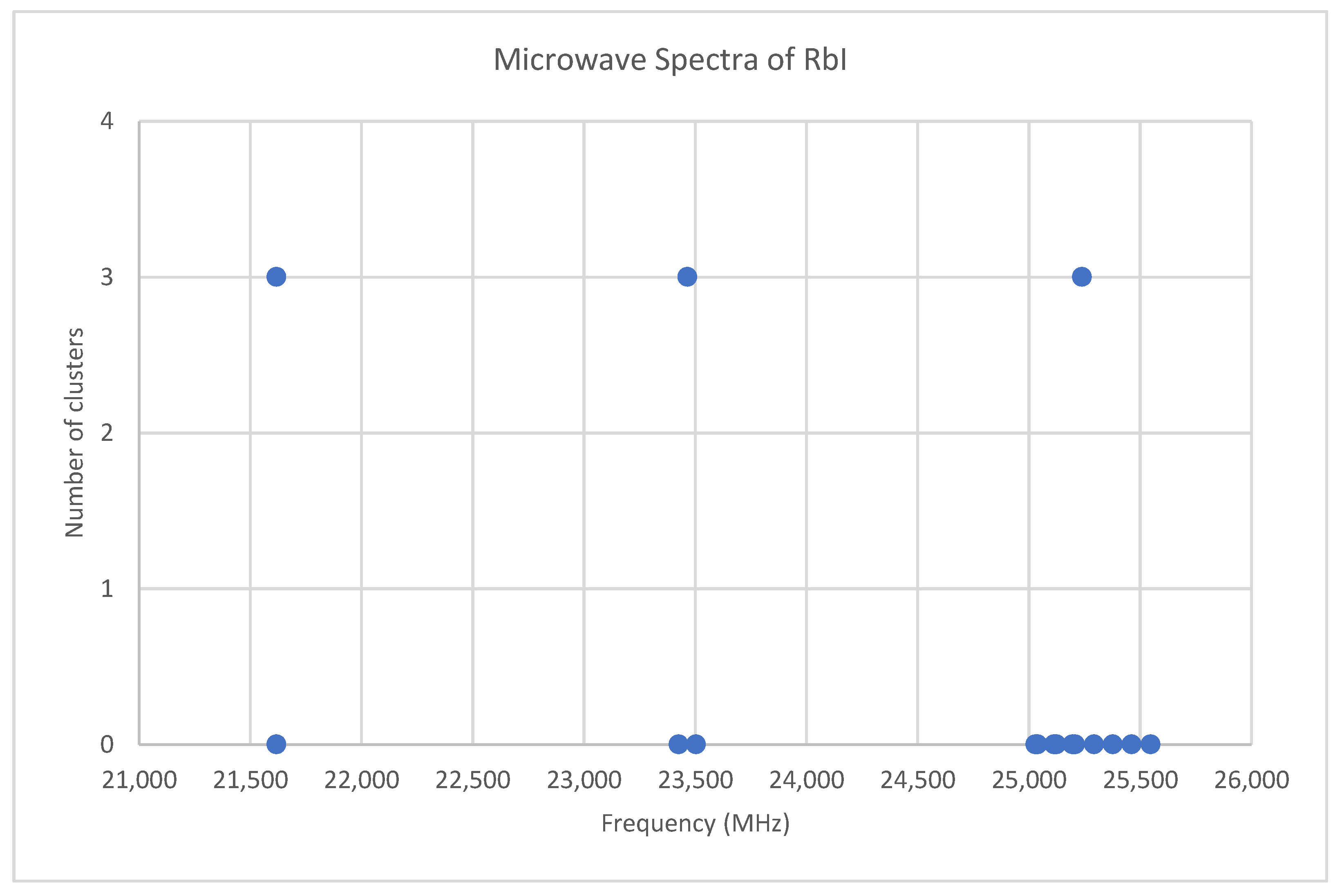
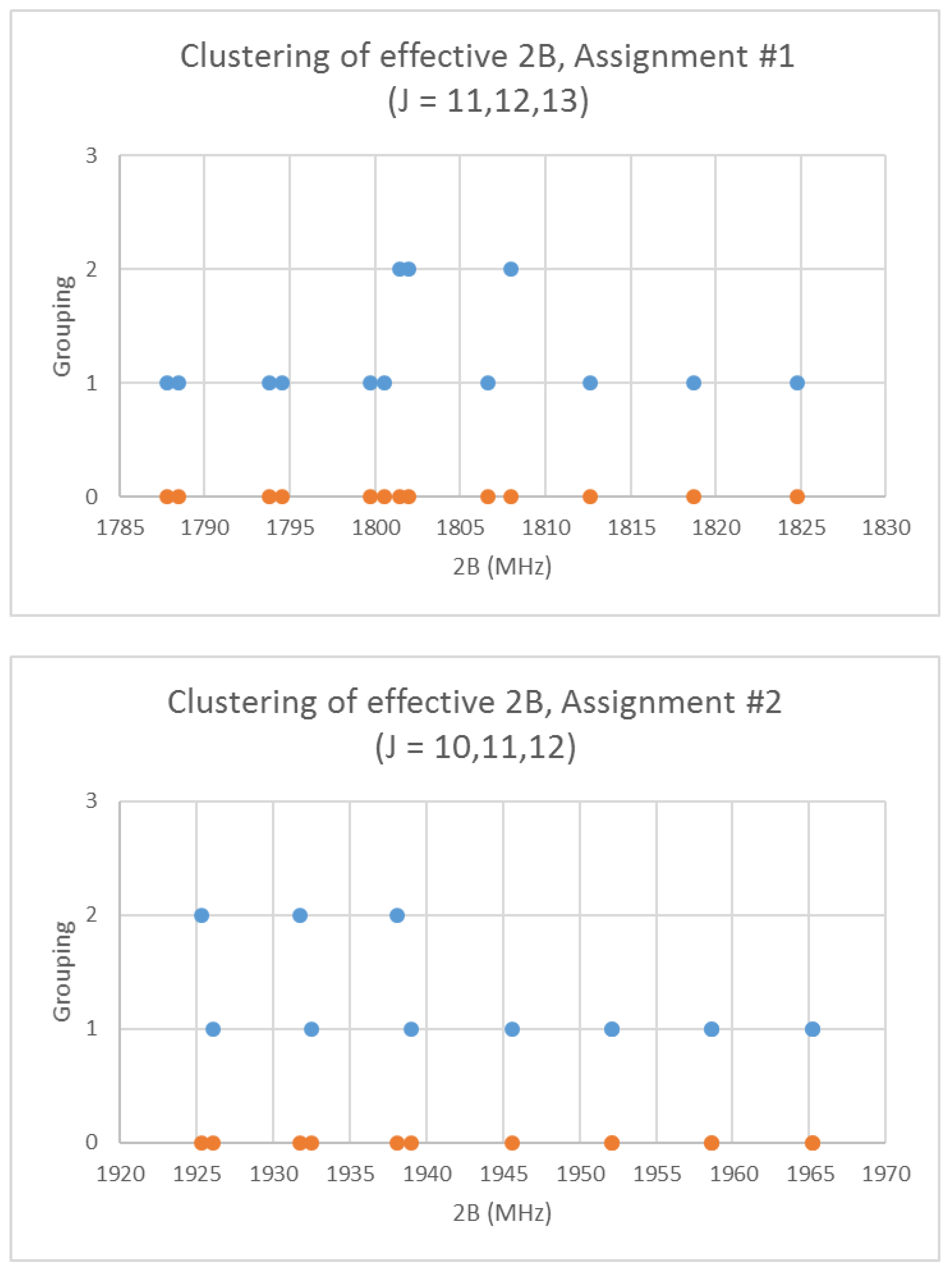
Rubidium has two isotopes, ⁸⁵Rb and ⁸⁷Rb, present in approximately a 3:1 ratio. The predicted value of 2B from electron diffraction is 1880 MHz (see Supplementary Materials, Excel file RbI.xlsx). The spectra of rubidium iodide in the region 21.5–25.6 GHz was measured [31] at 660 °C, and the frequencies observed (error 0.1–0.2 MHz) are given in Figure 10. Inspection of the 13 frequencies demonstrates that there appears to be three major groupings (clusters) of frequencies. The centers of the clusters are at 21,617.58, 23,464.75, and 25,238.83 MHz, with an average difference of 1810(37) MHz. The average difference between the highest frequency components is 1965(80) MHz. Using the estimated 2B or cluster averages would suggest either J = 10, 11, 12 (Assignment # 2) or J = 11, 12, 13 (Assignment #1), whereas using the highest frequency differences (assuming v = 0) would suggest J = 10, 11, 12, with an anomaly for J = 11. While the preference is for J = 10, 11, 12, the assignment is somewhat less definitive, so we have plotted the effective rotational constants for both scenarios (Figure 11). For assignment #1, all 13 points are still visible in nine subclusters, apparently in two vibrational progressions. This would imply that the centrifugal distortion constants are quite large, and that there are at least four points with the same v, but with multiple values of J. In addition, the B_e ratio is 1.009306. For assignment #2, only 10 clusters are visible, and these can (barely) be separated into two vibrational progressions with a B_e ratio of 1.013951. The expected mass ratio is 1.013961, which agrees with the second assignment to five significant figures. We therefore assume that the transitions are as assignment #2. The effective rotational constants for J = 11 correspond to v = 1–2, not to v = 0–1, which explains why the highest frequency method for J determination did not work as well.

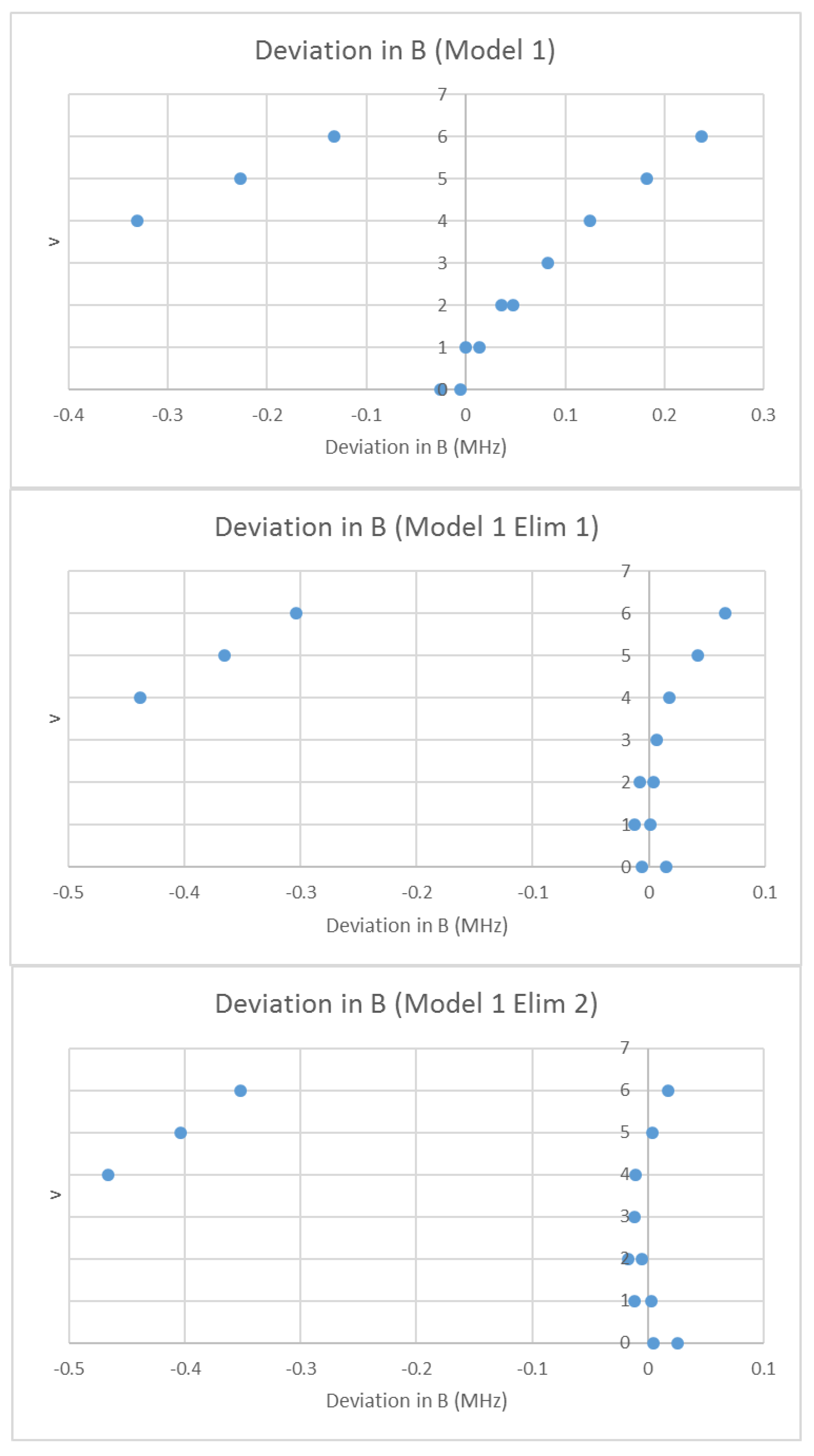
What would happen if we assumed that the spectrum was due to a single isotopologue, but that some lines were doubled due to some unknown effect? In that case, we may analyze the effective rotational constants as usual using Model 1. The residual error of this model is shown in Figure 12. There is a clear separation of the residual into two groups with this double assignment, and the least-squares process tries to fit both, resulting in a fairly large error. If we eliminate all points currently assigned to v = 4–6 (Model 1 Elim 1), the error drops significantly, and one set of the excluded points fits the expected residual error pattern. We can then re-include those points in the fit (Model 1 Elim 2). The points excluded belong to a second species. We then re-assign the vibrational quantum numbers of the second species to obtain a reasonable B_e ratio, from v = 4–6 (1.000736) to v = 0–2 (1.013950). We then proceed as usual to obtain r_e of 3.176993 and 3.176997 Å for the two isotopologues (

Table 5. Model parameters for rubidium iodide (MHz) (⁸⁵Rb¹²⁷I, n = 10; ⁸⁷Rb¹²⁷I, n = 3).

	Model	Be	αe	γe	De1	SSE
85Rb127I	1	984.221	3.261	n/a	n/a	1.013
	2	984.245	3.284	0.0033	n/a	0.237
	3	984.307	3.259	n/a	289	0.644
	4	984.236	3.279	0.0027	−81	0.113
87Rb127I	1	970.681	3.204	n/a	n/a	0.014
	2	970.672	3.188	−0.0056	n/a	exact

¹ Centrifugal distortion constants have been multiplied by 10⁶.

).

The pedagogical goals achieved here show that that, for RbI, (1) plotting effective rotational constants for different J assignments can assist in determining J, and (2) plotting residuals can help identify incorrect assumptions.

6.6. Rubidium Bromide (RbBr)

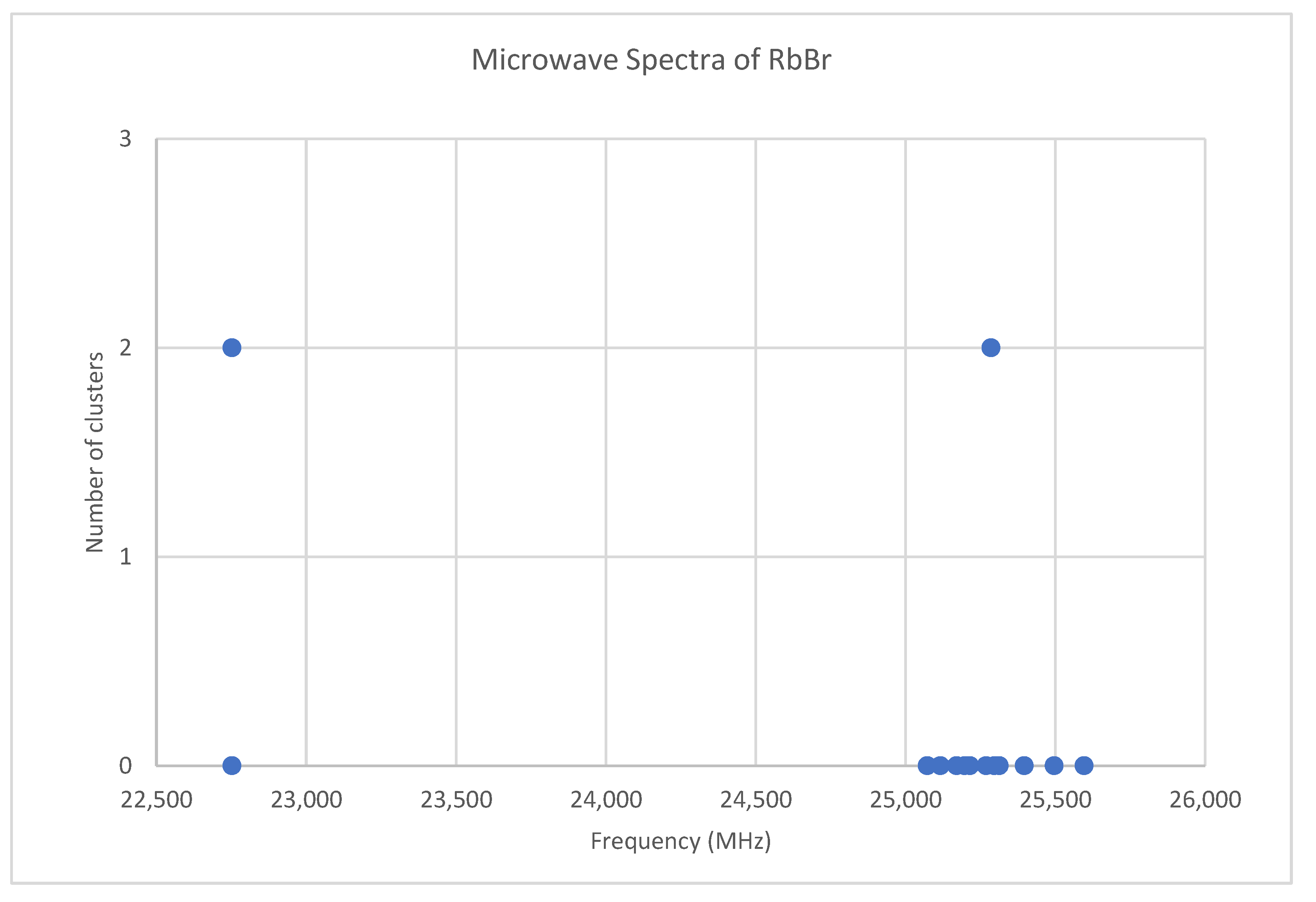
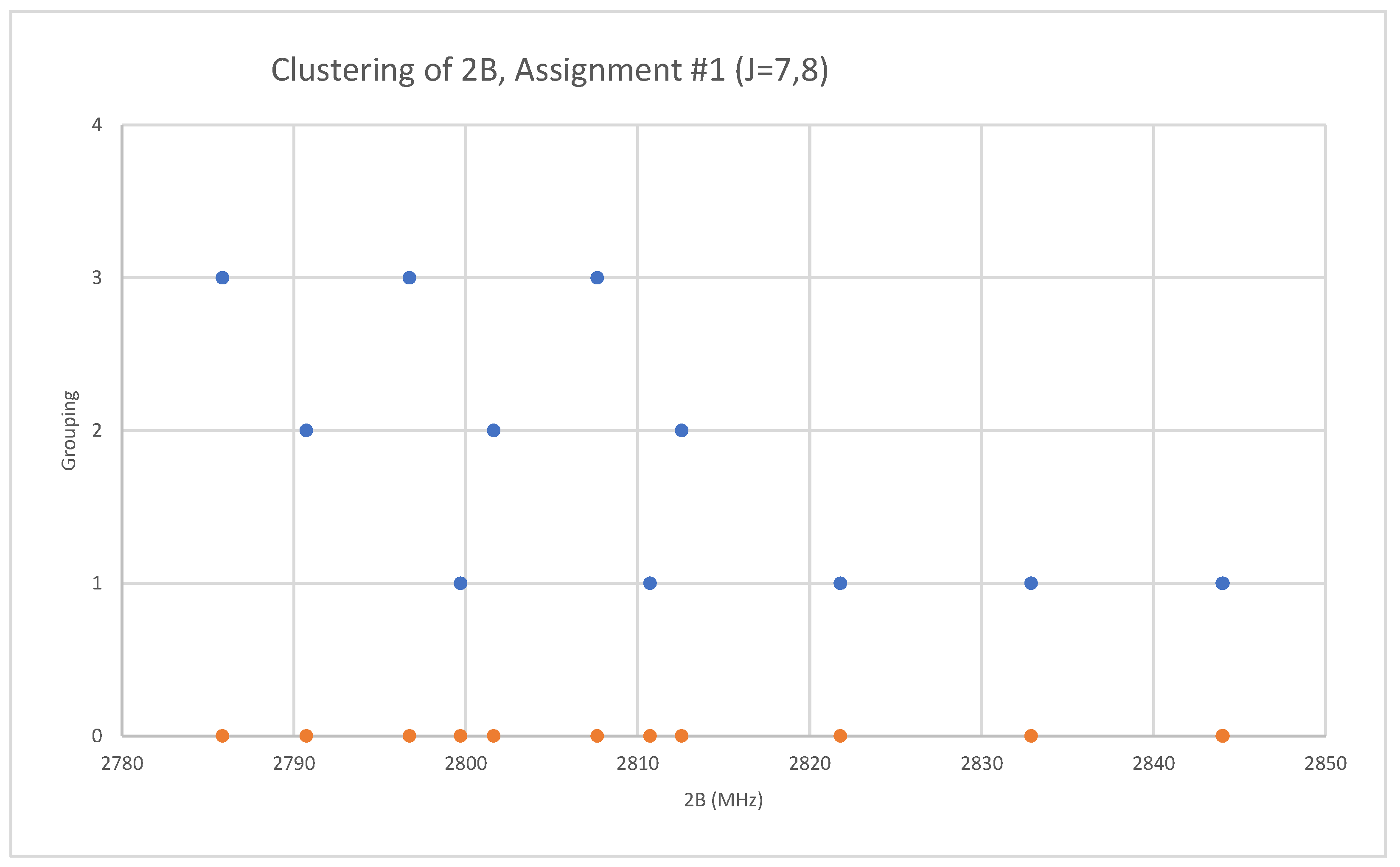
Because both rubidium and bromine are diisotopic, there may be a total of four isotopologues that could be observed. The predicted value of 2B from electron diffraction is 2650 MHz (see Supplementary Materials, Excel file RbBr.xlsx). The spectrum of rubidium bromide in the region 22.5–26.0 GHz was measured [31] at 730 °C, and the frequencies observed (error 0.1 MHz) are given in Figure 13. Inspection of the 12 frequencies demonstrates that there appear to be two major groupings (clusters) of frequencies, a single frequency at 22,752.29 MHz and a cluster centered at 25,285.29 MHz. The cluster difference is 2533 MHz, but the highest frequency components differ by 2843.70 MHz. Using the estimated 2B suggests either J = 7,8 or J = 8,9. Using the cluster average would suggest J = 8,9, whereas using the highest frequency differences (assuming v = 0) would suggest J = 7,8. With the highest frequency differences usually being more accurate, and along with the 2B clustering favoring this as well, we assign these to J = 7,8, with three different vibrational progressions (Figure 14).

The lightest isotopologue (⁸⁵Rb⁷⁹Br) is also the most abundant. The mass ratios for the heavier isotopologues are 1.011195 (⁸⁷Rb⁷⁹Br), 1.012963 (⁸⁵Rb⁸¹Br), and 1.024452 (⁸⁷Rb⁸¹Br). The B_e ratios for Model 1 are calculated as 1.011188 and 1.012955 and for Model 2 as 1.011202 and 1.012965, which demonstrate that the other two isotopologues observed are ⁸⁷Rb⁷⁹Br and ⁸⁵Rb⁸¹Br (

Table 6. Model parameters for rubidium bromide (MHz) (⁸⁵Rb⁷⁹Br, n = 6; ⁸⁷Rb⁷⁹Br, n = 3; ⁸⁵Rb⁸¹Br, n = 3).

	Model	Be	αe	γe	De1	SSE
85Rb79Br	1	1424.768	5.542	n/a	n/a	0.432
	2	1424.798	5.583	0.0086	n/a	0.041
	3	1424.822	5.538	n/a	−0.79	0.268
	4	1424.822	5.576	0.0076	−0.40	0.005
87Rb79Br	1	1409.003	5.456	n/a	n/a	0.011
	2	1409.014	5.478	0.0072	n/a	exact
85Rb81Br	1	1406.546	5.450	n/a	n/a	0.020
	2	1406.562	5.479	0.0097	n/a	exact

¹ Centrifugal distortion constants have been multiplied by 10⁶.

). The values of r_e are calculated as 2.944776, 2.944820, and 2.944823 Å.

The pedagogical goal achieved here shows that, for RbBr, more than two isotopologues can be successfully analyzed.

6.7. Potassium Iodide (KI)

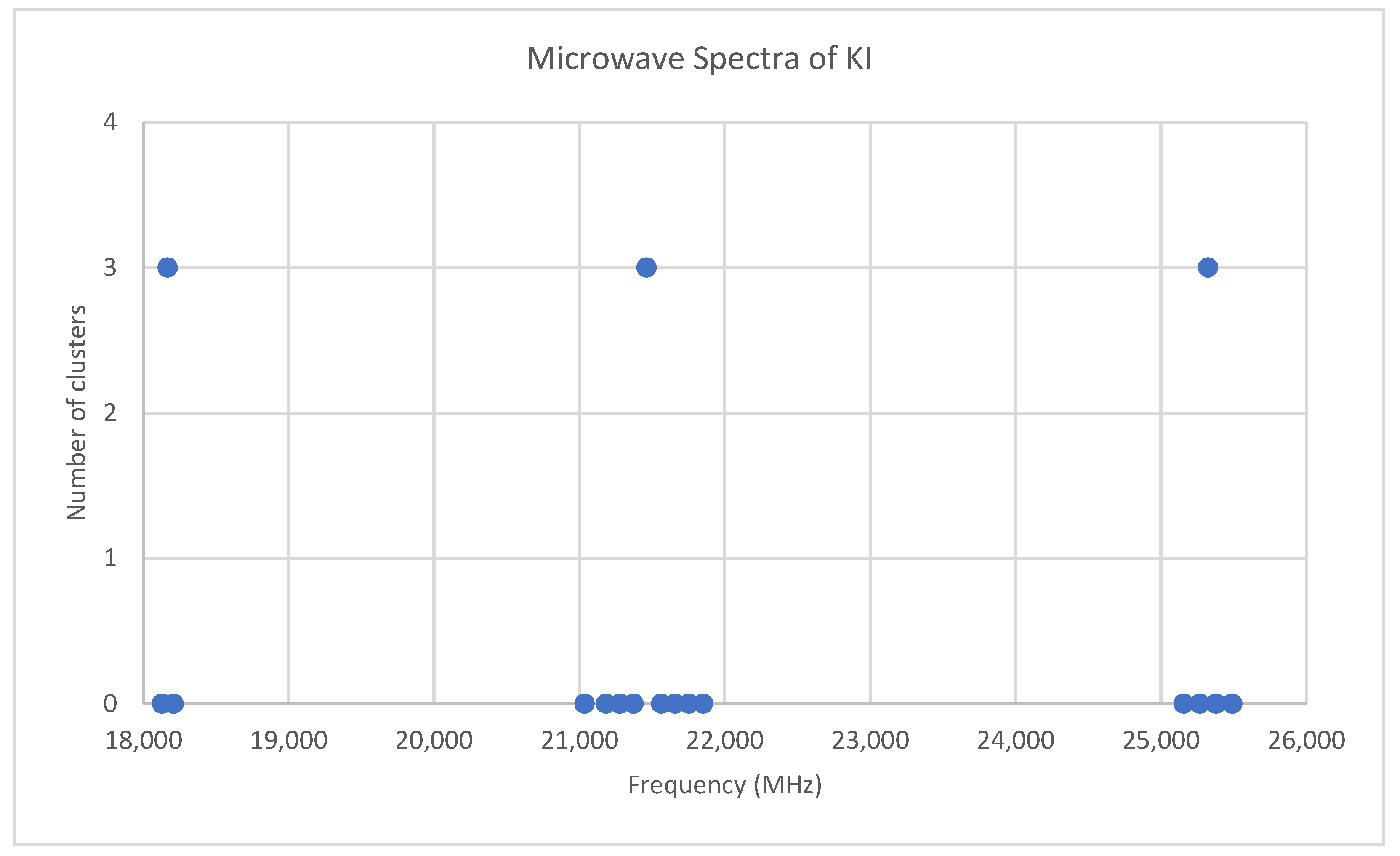
Potassium has two isotopes, ³⁹K and ⁴¹K, present in approximately a 14:1 ratio. The predicted value of 2B from electron diffraction is 3300 MHz (see Supplementary Materials, Excel file KI.xlsx). The spectrum of potassium iodide in the region 18–26 GHz was measured [31] at 690 °C, and the frequencies observed (error 0.1–0.3 MHz) are given in Figure 15. Inspection of the 14 frequencies demonstrates that there appears to be three major groupings (clusters) of frequencies. Analysis of this spectrum is left for the reader as a more challenging exercise (Appendix B). The results for ³⁹K¹²⁷I are Model 1, B_e = 1824.840, α_e = 7.941 MHz; Model 2, B_e = 1824.962, α_e = 8.047, γ_e = −0.0141 MHz; Model 3, B_e = 1825.023, α_e = 7.944, D_e = 0.0022 MHz; Model 4, B_e = 1825.059, α_e = 8.040, γ_e = −0.0130, D_e = 0.0013 MHz. The value of r_e is calculated as 3.047776 Å. The value of r₀ for the heavier isotopologue ⁴¹K¹²⁷I can be calculated as 3.051148 Å.

6.8. Potassium Chloride (KCl)

Potassium chloride has four naturally occurring isotopologues: ³⁹K³⁵Cl (70.65%), ³⁹K³⁷Cl (22.61%), ⁴¹K³⁵Cl (5.10%), ⁴¹K³⁷Cl (1.63%). The predicted value of 2B from electron diffraction is 7100 MHz (see Supplementary Materials, Excel file KCl.xlsx). The spectra of potassium chloride in the region 22.4–23.2 GHz was measured [39] at 715 °C, and the four frequencies observed (error 10 MHz) could either correspond to a vibrational progression, with a gap, or possibly to a mixture of up to four isotopologues. This determination is left to the reader (see Appendix C). A more precise spectrum was measured [40] at 700 °C and is also left as an exercise (see Appendix D).

6.9. Sodium Chloride (NaCl)

Sodium is monoisotopic. The predicted value of 2B from electron diffraction is 11,600 MHz (see Supplementary Materials, Excel file NaCl.xlsx). The spectrum of sodium chloride in the region 25.0–26.1 GHz was measured [38] at 775 °C, and the seven frequencies observed (error 0.75 MHz) correspond to two vibrational progressions. The assignment is left to the reader (Appendix E).

7. Conclusions

The microwave spectra of CO, CsI, CsBr, CsCl, CsF, RbI, RbBr, KI, KCl, and NaCl are presented and procedures for their analysis are discussed. By the use of either additional information (electron or X-ray diffraction) or by cluster analysis of the spectra, the approximate value of 2B can be determined, followed by the assignment of the frequencies to rotational quantum number J (Model 0). Once assigned, effective rotational constants for each transition can be assigned to specific vibrational quantum numbers v and/or isotopologues, to obtain the rotational constant B_e, bond length r_e, and vibration–rotation interaction constant α_e (Model 1). In some cases, other spectroscopic constants (D_e, γ_e) can be determined.

References

- Ewing, G.W. Microwave Absorption Spectroscopy. J. Chem. Educ. 1966, 43, A683–A722. [Google Scholar]
- Townes, C.H.; Schawlow, A.L. Microwave Spectroscopy; Dover: New York, NY, USA, 1975. [Google Scholar]
- Schwendeman, R.H.; Volltrauer, H.N.; Laurie, V.W.; Thomas, E.C. Microwave Spectroscopy in the Undergraduate Laboratory. J. Chem. Educ. 1970, 47, 526–532. [Google Scholar]
- Dyke, T.R.; Muenter, J.S. A Stark Modulation Absorption Cell for Student Microwave Spectrometers. J. Chem. Educ. 1974, 51, 33. [Google Scholar] [CrossRef]
- Pollnow, G.F.; Hopfinger, A.J. A Computer Experiment in Microwave Spectroscopy. J. Chem. Educ. 1968, 45, 528–531. [Google Scholar] [CrossRef]
- Pollnow, G.F.; Chung, C.S.C. An Interactive Computer Program for Microwave Spectroscopy. J. Chem. Educ. 1973, 50, 794. [Google Scholar]
- McNaught, I.J.; Moore, R. Microwave Spectroscopy Tutor. J. Chem. Educ. 1995, 72, 993–994. [Google Scholar] [CrossRef]
- McNaught, I.J.; Moore, R. Winspec: A Microwave Spectroscopy Tutor. J. Chem. Educ. 1996, 73, 523.az. [Google Scholar]
- Woods, R.; Henderson, G. FTIR Rotational Spectroscopy. J. Chem. Educ. 1987, 64, 921–924. [Google Scholar] [CrossRef]
- McQuarrie, D.A. Quantum Chemistry, 2nd ed.; University Science Books: Herndon, VA, USA, 2008; Chapter 6. [Google Scholar]
- Pye, C.C. On the Solution of the Quantum Rigid Rotor. J. Chem. Educ. 2006, 83, 460–463. [Google Scholar] [CrossRef]
- Moynihan, C.T. Rationalization of the ΔJ=±1 Selection Rule for Rotational Transitions. J. Chem. Educ. 1969, 46, 431. [Google Scholar]
- Foss, J.G. Photonic Angular Momentum and Selection Rules for Rotational Transitions. J. Chem. Educ. 1970, 47, 778–779. [Google Scholar] [CrossRef]
- Chattaraj, P.K.; Sannigrahi, A.B. A Simple Group-Theoretical Derivation of the Selection Rules for Rotational Transitions. J. Chem. Educ. 1990, 67, 653–655. [Google Scholar]
- Laidler, K.J.; Meiser, J.H. Physical Chemistry, 3rd ed.; Houghton Mifflin: Boston, MA, USA, 1999; Chapter 13. [Google Scholar]
- Engel, T.; Reid, P. Physical Chemistry; Pearson: San Francisco, CA, USA, 2006; Chapter 19. [Google Scholar]
- House, J.E. Fundamentals of Quantum Mechanics; Academic Press: San Diego, CA, USA, 1998; Chapter 7. [Google Scholar]
- Ratner, M.A.; Schatz, G.C. Introduction to Quantum Mechanics in Chemistry; Prentice-Hall: Upper Saddle River, NJ, USA, 2001; Chapter 4. [Google Scholar]
- Atkins, P.; de Paula, J. Physical Chemistry, 10th ed.; Freeman: New York, NY, USA, 2014; Chapter 12. [Google Scholar]
- Berry, R.S.; Rice, S.A.; Ross, J. Physical Chemistry, 2nd ed.; Oxford University Press: New York, NY, USA, 2000; Chapter 7. [Google Scholar]
- Alberty, R.A.; Silbey, R.J. Physical Chemistry, 2nd ed.; Wiley: New York, NY, USA, 1997; Chapter 13. [Google Scholar]
- Mortimer, R.G. Physical Chemistry, 2nd ed.; Harcourt: San Diego, CA, USA, 2000; Chapter 19. [Google Scholar]
- Zielinski, T.J. Fostering Creativity and Learning Using Instructional Symbolic Mathematics Documents. J. Chem. Educ. 2009, 86, 1466–1467. [Google Scholar]
- Microsoft Office Professional Plus (Excel) 2016, Microsoft Corporation: Redmond, WA, USA, 2016.
- Solver, Microsoft Office Add-In, Frontline Systems: Incline Village, NV, USA, 2016.
- Gilliam, O.R.; Johnson, C.M.; Gordy, W. Microwave Spectroscopy in the Region from Two to Three Millimeters. Phys. Rev. 1950, 78, 140–144. [Google Scholar]
- Vegard, L. Struktur und Leuchtfahigkeit von festem Kohlenoxyd. Z. Phys. 1930, 61, 185–190. [Google Scholar] [CrossRef]
- Crystallography Open Database. Available online: http://www.crystallography.net (accessed on 31 March 2018).
- Wyckoff, R.W.G. Crystal Structures; Wiley: New York, NY, USA, 1963; Chapter 3; pp. 85–237. [Google Scholar]
- Maxwell, L.R.; Hendricks, S.B.; Mosley, V.M. Interatomic Distances of the Alkali Halide Molecules by Electron Diffraction. Phys. Rev. 1937, 52, 968–972. [Google Scholar]
- Honig, A.; Mandel, M.; Stitch, M.L.; Townes, C.H. Microwave Spectra of the Alkali Halides. Phys. Rev. 1954, 96, 629–642. [Google Scholar] [CrossRef]
- Pye, C.C. One-Dimensional Cluster Analysis and its Application to Chemistry. Chem. Educ. 2020, 25, 50–57. [Google Scholar]
- Pye, C.C. Intuitive Solution to Quantum Harmonic Oscillator at Infinity. J. Chem. Educ. 2004, 81, 830–831. [Google Scholar]
- McHale, J.L. Molecular Spectroscopy; Prentice-Hall: Upper Saddle River, NJ, USA, 1999; Chapters 8–9. [Google Scholar]
- Dykstra, C.E. Introduction to Quantum Chemistry; Prentice-Hall: Englewood Cliffs, NJ, USA, 1994; Chapter 5. [Google Scholar]
- Hollenberg, J.L. Energy States of Molecules. J. Chem. Educ. 1970, 47, 2–14. [Google Scholar] [CrossRef]
- Brown, J.M. Molecular Spectroscopy; Oxford Science Publications: Oxford, UK, 1999; Chapter 5. [Google Scholar]
- Stitch, M.L.; Honig, A.; Townes, C.H. Microwave Spectra at High Temperature—Spectra of CsCl and NaCl. Phys. Rev. 1952, 86, 813–814. [Google Scholar] [CrossRef]
- Stitch, M.L.; Honig, A.; Townes, C.H. High Temperature Microwave Spectroscopy—Spectrum of KCl, TlCl. Phys. Rev. 1952, 86, 607. [Google Scholar]
- Tate, P.A.; Strandberg, M.W.P. Stark Effect in the Microwave Spectra of KCl and NaCl. J. Chem. Phys. 1954, 22, 1380–1383. [Google Scholar] [CrossRef]
Figure 1.
The spectrum of cesium iodide (Grouping 0), and the cluster averages for k = 3.
Figure 2.
The effective rotational constants (×2) of cesium iodide.
Figure 3.
The residual plots of four different models for the microwave spectrum of cesium iodide.
Figure 4.
The microwave spectrum of cesium bromide, and the 3-cluster averages.
Figure 5.
The effective rotational constants (×2) of cesium bromide. Different J values are offset by 0.2 units. The orange points are the original spectrum, the blue points are separation into isotopologues.
Figure 6.
The deviation from Model 1 for 133Cs79Br.
Figure 7.
The microwave spectrum of cesium chloride, and separation into isotopologues. The orange points are the original spectrum, the blue points are separation into isotopologues.
Figure 8.
Comparison of microwave spectra of cesium chloride from two sources (Grouping 0 (orange) [38], Grouping 1 (blue) [31]).
Figure 9.
The microwave spectrum of cesium fluoride.
Figure 10.
The microwave spectrum of rubidium iodide, and the 3-cluster averages.
Figure 11.
The rotational constants of rubidium iodide for two different J assignments. The orange points are the original spectrum, the blue points are separation into isotopologues.
Figure 12.
The Model 1 residuals of the effective rotational constants of rubidium iodide, assuming a single species. The top graph includes all points, the middle graph eliminates points assigned as v = 4–6 from the fit, and the bottom graph only eliminates the leftmost v = 4–6 points.
Figure 13.
The microwave spectrum of rubidium bromide, and the 2-cluster averages.
Figure 14.
The rotational constants of rubidium bromide. The orange points are the original spectrum, the blue points are separation into isotopologues.
Figure 15.
The microwave spectrum of potassium iodide, and the 3-cluster averages.